Peak shape quality: beta parameters

Calculate beta parameters for a chromatographic peak, both its similarity to a bell curve of varying degrees of skew (i.e., assymmetry or tailing factor) and the standard deviation of the residuals after the best-fit bell is normalized and subtracted. This function requires at least 5 scans or it will return NA for both parameters.

Usage

betaValues(
  intensity = numeric(),
  rtime = seq_along(intensity),
  skews = c(3, 3.5, 4, 4.5, 5),
  zero.rm = TRUE
)

Arguments

intensity: A numeric vector corresponding to the peak intensities with a minimum length of 5.
rtime: A numeric vector corresponding to the retention times of each intensity. Retention times are expected to be in increasing order without duplicates. If not provided, intensities will be assumed to be equally spaced.
skews: A numeric vector of the skews to try. These values will be passed to shape1 parameter of the dbeta() function (with its shape2 parameter set to 5). Values less than 5 will generated increasingly right-skewed curves, while values greater than 5 will result in left-skewed curves. See Figure 8 in the original manuscript for visual examples.
zero.rm: logical(1) controlling whether missing scans are dropped prior to curve fitting. The default, zero.rm = TRUE, will remove intensities of zero or NA.

Value

numeric of length 2.

Details

The function compares the actual chromatographic peak to Beta distribution curves calculated with the dbeta() function.

References

Kumler W, Hazelton B J and Ingalls A E (2023) "Picky with peakpicking: assessing chromatographic peak quality with simple metrics in metabolomics" BMC Bioinformatics 24(1):404. doi: 10.1186/s12859-023-05533-4

Author

William Kumler

Examples


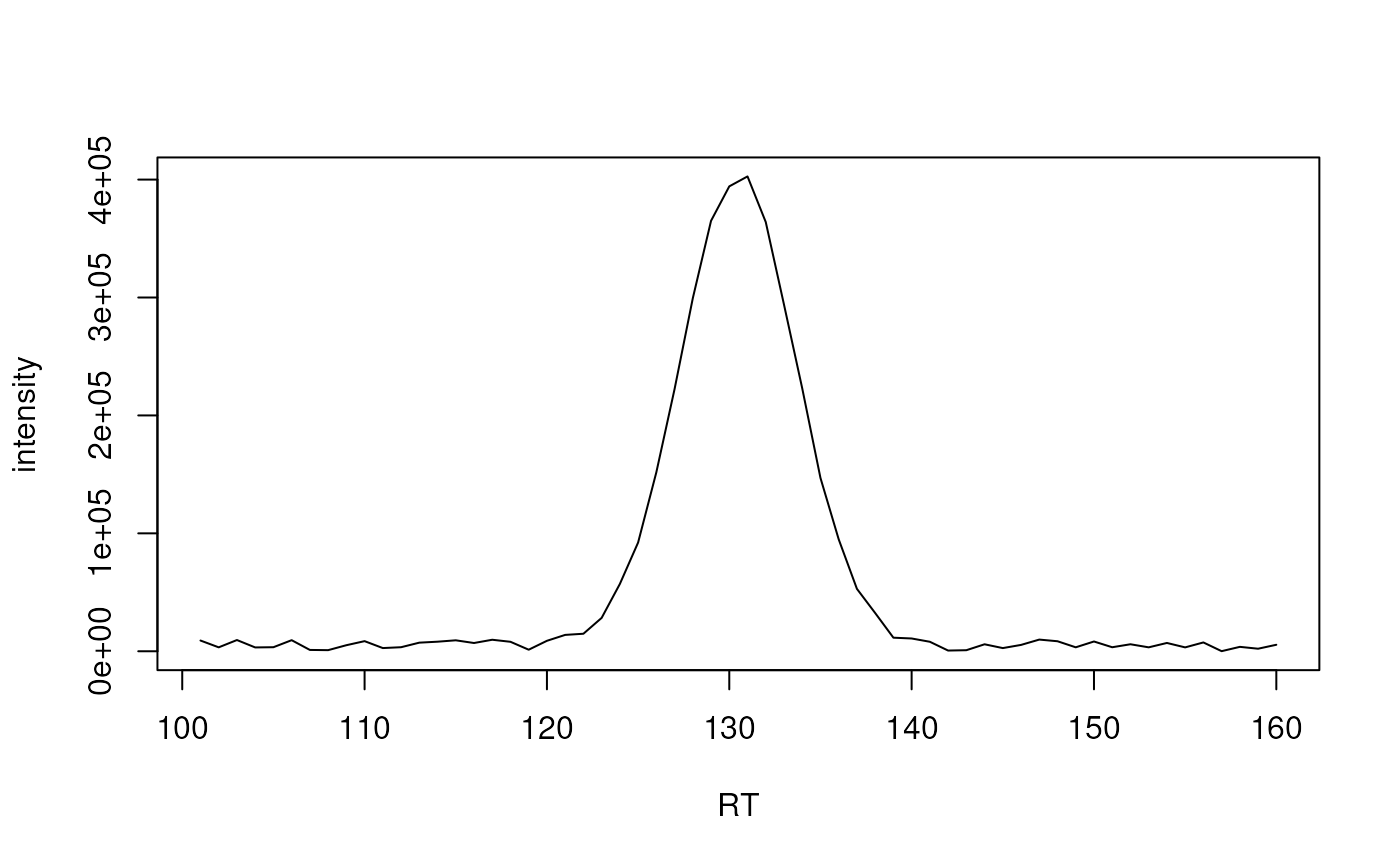
## Define intensity values of a typical chromatographic peak
skinny_peak <- c(9107, 3326, 9523, 3245, 3429, 9394, 1123, 935, 5128, 8576,
                 2711, 3427, 7294, 8109, 9288, 6997, 9756, 8034, 1317, 8866,
                 13877, 14854, 28296, 57101, 92209, 151797, 222386, 299402,
                 365045, 394255, 402680, 363996, 293985, 222989, 147007,
                 94947, 52924, 32438, 11511, 10836, 8046, 601, 889, 5917,
                 2690, 5381, 9901, 8494, 3349, 8283, 3410, 5935, 3332,
                 7041, 3284, 7478, 76, 3739, 2158, 5507)
skinny_peak_rt <- seq_along(skinny_peak)+100

plot(skinny_peak_rt, skinny_peak, xlab = "RT",
    ylab = "intensity", type = "l")


## Calculate beta parameters for the full region including noise signal
## around the peak
res <- betaValues(skinny_peak, skinny_peak_rt)
res
#> best_cor beta_snr 
#> 0.727437 6.789728 

## Calculate beta parameters for peak signal
res <- betaValues(skinny_peak[20:40], skinny_peak_rt[20:40])
res
#>  best_cor  beta_snr 
#> 0.9858619 7.1275735 

## Define noisy chromatographic signal
noise_peak <- c(0.288, 0.788, 0.409, 0.883, 0.94, 0.046, 0.528, 0.892,
                0.551, 0.457, 0.957, 0.453, 0.678, 0.573, 0.103, 0.9,
                0.246, 0.042, 0.328, 0.955, 0.89, 0.693, 0.641, 0.994,
                0.656, 0.709, 0.544, 0.594, 0.289, 0.147, 0.963, 0.902,
                0.691, 0.795, 0.025, 0.478, 0.758, 0.216, 0.318, 0.232,
                0.143, 0.415, 0.414, 0.369, 0.152, 0.139, 0.233, 0.466,
                0.266, 0.858, 0.046, 0.442, 0.799, 0.122, 0.561, 0.207,
                0.128, 0.753, 0.895, 0.374, 0.665, 0.095, 0.384, 0.274,
                0.815, 0.449, 0.81, 0.812, 0.794, 0.44, 0.754, 0.629, 0.71,
                0.001, 0.475, 0.22, 0.38, 0.613, 0.352, 0.111, 0.244, 0.668,
                0.418, 0.788, 0.103, 0.435, 0.985, 0.893, 0.886, 0.175,
                0.131, 0.653, 0.344, 0.657, 0.32, 0.188, 0.782, 0.094,
                0.467, 0.512)
noise_peak_rt <- seq_along(noise_peak) + 10
res <- betaValues(noise_peak, noise_peak_rt)
res
#>    best_cor    beta_snr 
#> -0.03291661  0.39695171