Linear model-based normalization of abundance matrices

The fit_lm and adjust_lm functions facilitate linear model-based normalization of abundance matrices. The expected noise in a numeric data matrix can be modeled with a linear regression model using the fit_lm function and the data can subsequently be adjusted using the adjust_lm function (i.e., the modeled noise will be removed from the abundance values). A typical use case would be to remove injection index dependent signal drifts in a LC-MS derived metabolomics data: a linear model of the form y ~ injection_index could be used to model the measured abundances of each feature (each row in a data matrix) as a function of the injection index in which a specific sample was measured during the LC-MS measurement run. The fitted linear regression models can subsequently be used to adjust the abundance matrix by removing these dependencies from the data. This allows to perform signal adjustments as described in (Wehrens et al. 2016).

The two functions are described in more details below:

fit_lm allows to fit a linear regression model (defined with parameter formula) to each row of the numeric data matrix submitted with parameter y. Additional covariates of the linear model defined in formula are expected to be provided as columns in a data.frame supplied via the data parameter.

The linear model is expected to be defined by a formula starting with y ~ . To model for example an injection index dependency of values in y a formula y ~ injection_index could be used, with values for the injection index being provided as a column "injection_index" in the data data frame. fit_lm would thus fit this model to each row of y.

Linear models can be fitted either with the standard least squares of lm() by setting method = "lm" (the default), or with the more robust methods from the robustbase package with method = "lmrob".

adjust_lm can be used to adjust abundances in a data matrix y based on linear regression models provided with parameter lm. Parameter lm is expected to be a list of length equal to the number of rows of y, each element being a linear model (i.e., a results from lm or lmrob). Covariates for the model need to be provided as columns in a data.frame provided with parameter data. The number of rows of that data.frame need to match the number of columns of y. The function returns the input matrix y with values in rows adjusted with the linear models provided by lm. No adjustment is performed for rows for which the respective element in lm is NA. See examples below for details or the vignette for more examples, descriptions and information.

Usage

fit_lm(
  formula,
  data,
  y,
  method = c("lm", "lmrob"),
  control = NULL,
  minVals = ceiling(nrow(data) * 0.75),
  model = TRUE,
  ...,
  BPPARAM = SerialParam()
)

adjust_lm(y = matrix(), data = data.frame(), lm = list(), ...)

Arguments

formula: formula defining the model that should be fitted to the data. See also lm() for more information. Formulas should begin with y ~ as values in rows of y will be defined as y. See description of the fit_lm function for more information.
data: data.frame containing the covariates for the linear model defined by formula (for fit_lm) or used in lm (for adjust_lm). The number of rows has to match the number of columns of y.
y: for fit_lm: matrix of abundances on which the linear model pefined with formula should be fitted. For adjust_lm: matrix of abundances that should be adjusted using the models provided with parameter lm.
method: character(1) defining the linear regression function that should be used for model fitting. Can be either method = "lm" (the default) for standard least squares model fitting or method = "lmrob" for a robust alternative defined in the robustbase package.
control: a list speficying control parameters for lmrob. Only used if method = "lmrob". See help of lmrob.control in the robustbase package for details. By default control = NULL the KS2014 settings are used and scale-finding iterations are increased to 10000.
minVals: numeric(1) defining the minimum number of non-missing values (per feature/row) required to perform the model fitting. For rows in y for which fewer non-NA values are available no model will be fitted and a NA will be reported instead.
model: logical(1) whether the model frame are included in the returned linear models. Passed to the lm or lmrob functions.
...: for fit_lm: additional parameters to be passed to the downstream calls to lm or lmrob. For adjust_lm: ignored.
BPPARAM: parallel processing setup. See bpparam() for more information. Parallel processing can improve performance especially for method = "lmrob".
lm: list of linear models (as returned by lm or lmrob) such as returned by the fit_lm function. The length of the list is expected to match the number of rows of y, i.e., each element should be a linear model to adjust the specific row, or NA to skip adjustment for that particular row in y.

Value

For `fit_lm`: a `list` with linear models (either of type *lm* or
*lmrob*) or length equal to the number of rows of `y`. `NA` is
reported for rows with too few non-missing data points (depending
on parameter `minValues`).
For `adjust_lm`: a numeric matrix (same dimensions as input matrix
`y`) with the values adjusted with the provided linear models.

References

Wehrens R, Hageman JA, van Eeuwijk F, Kooke R, Flood PJ, Wijnker E, Keurentjes JJ, Lommen A, van Eekelen HD, Hall RD Mumm R and de Vos RC. Improved batch correction in untargeted MS-based metabolomics. Metabolomics 2016; 12:88.

Author

Johannes Rainer

Examples


## See also the vignette for more details and examples.

## Load a test matrix with abundances of features from a LC-MS experiment.
vals <- read.table(system.file("txt", "feature_values.txt",
                                package = "MetaboCoreUtils"), sep = "\t")
vals <- as.matrix(vals)

## Define a data.frame with the covariates to be used to model the noise
sdata <- data.frame(injection_index = seq_len(ncol(vals)))

## Fit a linear model describing the feature abundances as a
## function of the index in which samples were injected during the LC-MS
## run. We're fitting the model to log2 transformed data.
## Note that such a model should **only** be fitted if the samples
## were randomized, i.e. the injection index is independent of any
## experimental covariate. Alternatively, the injection order dependent
## signal drift could be estimated using QC samples (if they were
## repeatedly injected) - see vignette for more details.
ii_lm <- fit_lm(y ~ injection_index, data = sdata, y = log2(vals))

## The result is a list of linear models
ii_lm[[1]]
#> 
#> Call:
#> lm(formula = formula, data = data, model = model)
#> 
#> Coefficients:
#>     (Intercept)  injection_index  
#>       14.833410         0.001587  
#> 

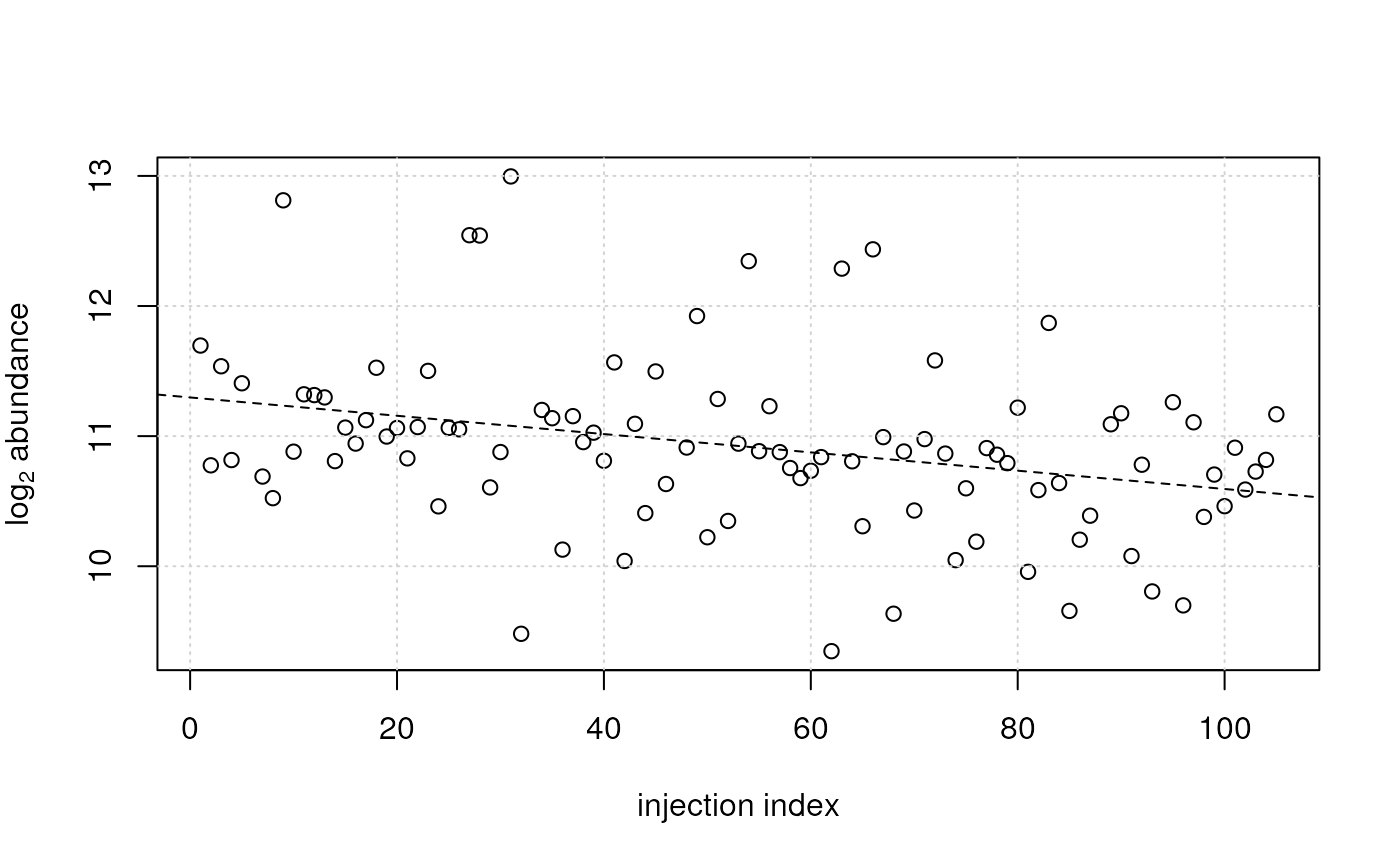
## Plotting the data for one feature:
plot(x = sdata$injection_index, y = log2(vals[2, ]),
    ylab = expression(log[2]~abundance), xlab = "injection index")
grid()
## plot also the fitted model
abline(ii_lm[[2]], lty = 2)


## For this feature (row) a decreasing signal intensity with injection
## index was observed (and modeled).

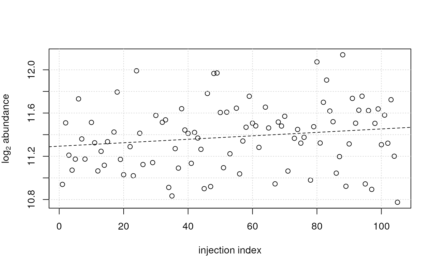
## For another feature an increasing intensity can be observed.
plot(x = sdata$injection_index, y = log2(vals[3, ]),
    ylab = expression(log[2]~abundance), xlab = "injection index")
grid()
## plot also the fitted model
abline(ii_lm[[3]], lty = 2)


## This trend can be removed from the data using the `adjust_lm` function
## by providing the linear models descring the drift. Note that, because
## we're adjusting log2 transformed data, the resulting abundances are
## also in log2 scale.
vals_adj <- adjust_lm(log2(vals), data = sdata, lm = ii_lm)

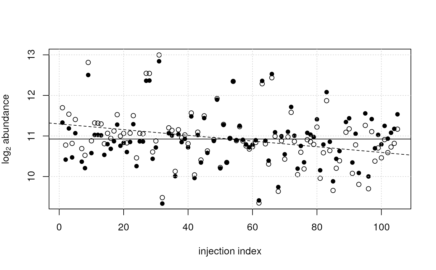
## Plotting the data before (open circles) and after adjustment (filled
## points)
plot(x = sdata$injection_index, y = log2(vals[2, ]),
    ylab = expression(log[2]~abundance), xlab = "injection index")
points(x = sdata$injection_index, y = vals_adj[2, ], pch = 16)
grid()
## Adding the line fitted through the raw data
abline(ii_lm[[2]], lty = 2)
## Adding a line fitted through the adjusted data
abline(lm(vals_adj[2, ] ~ sdata$injection_index), lty = 1)

## After adjustment there is no more dependency on injection index.