Using and understanding a Chromatograms object
Source:vignettes/using-a-chromatograms-object.Rmd
using-a-chromatograms-object.RmdPackage: Chromatograms 1.3.0
Compiled: Sat May 23 14:11:31 2026
Introduction
The Chromatograms package provides a scalable and flexible
infrastructure to represent, retrieve, and handle chromatographic data.
The Chromatograms object offers a standardized interface to
access and manipulate chromatographic data while supporting various ways
to store and retrieve this data through the concept of exchangeable
backends. This vignette provides general examples and
descriptions for the Chromatograms package.
Contributions to this vignette (content or correction of typos) or requests for additional details and information are highly welcome, ideally via pull requests or issues on the package’s github repository.
This vignette describe the structure of a Chromatograms object and
the methods that need to be implemented. In order to see the structure
of the object, the @ accessor is used to access the
different slots. This is possible because the Chromatograms
class is defined as an S4 class. However users should not use the
@ accessor to access the data stored in a
Chromatograms object, but instead use the methods defined
by the Chromatograms class.
Installation
The package can be installed with the BiocManager package.
To install BiocManager, use
install.packages("BiocManager"), and after that, use
BiocManager::install("Chromatograms") to install
Chromatograms.
The Chromatograms object
The Chromatograms object is a container for
chromatographic data, which includes peaks data (retention time
and related intensity values, also
referred to as peaks data variables in the context of
Chromatograms) and metadata of individual chromatograms
(so-called chromatogram variables). While a core set of
chromatogram variables (the coreChromatogramsVariables())
and peaks data variables (the corePeaksVariables()) are
guaranteed to be provided by a Chromatograms, it is
possible to add arbitrary variables to a Chromatograms
object.
The Chromatograms object is designed to contain
chromatographic data for a (large) set of chromatograms. The data is
organized linearly and can be thought of as a list of
chromatograms, where each element in the Chromatograms is
one chromatogram.
Available backends
Backends allow to use different backends to store
chromatographic data while providing via the
Chromatograms class a unified interface to use that data.
The Chromatograms package defines a set of example backends
but any object extending the base ChromBackend class could
be used instead. The default backends are:
ChromBackendMemory: the default backend to store data in memory. Due to its design theChromBackendMemoryprovides fast access to the peaks data and metadata. Since all data is kept in memory, this backend has a relatively large memory footprint (depending on the data) and is thus not suggested for very large experiments.ChromBackendMzR: this backend keeps only the chromatographic metadata variables in memory and relies on the mzR package to read chromatographic peaks (retention time and intensity values) from the original mzML files on-demand.ChromBackendSpectra: this backend generates chromatographic data from aSpectraobject. It can be used to create Total Ion Chromatograms (TIC), Base Peak Chromatograms (BPC), or Extracted Ion Chromatograms (EICs). It supports both in-memory and file-backedSpectraobjects. The backend uses factorization to group spectra into chromatograms based on variables like MS level and data origin (see details below).
All backends provide a consistent interface through the
Chromatograms object, regardless of where or how the data
is stored. The ChromBackendSpectra has a special feature:
it uses an internal sort index (spectraSortIndex) to
maintain retention time order without physically reordering the
underlying Spectra object. This is particularly important
for disk-backed Spectra objects, as it avoids loading all
data into memory. The sort index is automatically maintained during
subsetting and factorization operations.
Chromatographic peaks data
The peaks data variables information in the
Chromatograms object can be accessed using the
peaksData() function. peaksData can be
accessed, replaced, and also filtered/subsetted.
The core peaks data variables all have their own accessors and are as follows:
-
rtime: Anumericvector containing retention time values. -
intensity: Anumericvector containing intensity values.
Chromatograms metadata
The metadata of individual chromatograms (so called chromatograms
variables), can be accessed using the chromData()
function. The chromData can be accessed, replaced, and
filtered.
The core chromatogram variables all have their own accessor
methods, and it is guaranteed that a value is returned by them (or
NA if the information is not available).
The core variables and their data types are (alphabetically ordered):
-
chromIndex: anintegerwith the index of the chromatogram in the original source file (e.g., mzML file). -
collisionEnergy: for SRM data,numericwith the collision energy of the precursor. -
dataOrigin: optionalcharacterwith the origin of a chromatogram. -
storageLocation:characterdefining where the data is (currently) stored. -
msLevel:integerdefining the MS level of the data. -
mz: optionalnumericwith the (target) m/z value for the chromatographic data. -
mzMin: optionalnumericwith the lower m/z value of the m/z range in case the data (e.g., an extracted ion chromatogram EIC) was extracted from aChromtagoramsobject. -
mzMax: optionalnumericwith the upper m/z value of the m/z range. -
precursorMz: for SRM data,numericwith the target m/z of the precursor (parent). -
precursorMzMin: for SRM data, optionalnumericwith the lower m/z of the precursor’s isolation window. -
precursorMzMax: for SRM data, optionalnumericwith the upper m/z of the precursor’s isolation window. -
productMz: for SRM data,numericwith the target m/z of the product ion. -
productMzMin: for SRM data, optionalnumericwith the lower m/z of the product’s isolation window. -
productMzMax: for SRM data, optionalnumericwith the upper m/z of the product’s isolation window.
For details on the individual variables and their getter/setter
functions, see the help for Chromatograms
(?Chromatograms). Also, note that these variables are
suggested but not required to characterize a chromatogram.
Creating Chromatograms objects
The simplest way to create a Chromatograms object is by
defining a backend ofchoice, which mainly depends on what type of data
you have, and passing that to the Chromatograms constructor
function. Below we create such an object for a set of 2 chromatograms,
providing their metadata through a data.frame with the MS level, m/z,
and chromatogram index columns, and peaks data. The metadata includes
the MS level, m/z, and chromatogram index, while the peaks data includes
the retention time and intensity in a list of data.frames.
# A data.frame with chromatogram variables.
cdata <- data.frame(
    msLevel = c(1L, 1L),
    mz = c(112.2, 123.3),
    chromIndex = c(1L, 2L)
)

# Retention time and intensity values for each chromatogram.
pdata <- list(
    data.frame(
        rtime = c(11, 12.4, 12.8, 13.2, 14.6, 15.1, 16.5),
        intensity = c(50.5, 123.3, 153.6, 2354.3, 243.4, 123.4, 83.2)
    ),
    data.frame(
        rtime = c(45.1, 46.2, 53, 54.2, 55.3, 56.4, 57.5),
        intensity = c(100, 180.1, 300.45, 1400, 1200.3, 300.2, 150.1)
    )
)

# Create and initialize the backend
be <- backendInitialize(ChromBackendMemory(),
    chromData = cdata, peaksData = pdata
)

# Create Chromatograms object
chr <- Chromatograms(be)
chr
## Chromatographic data (Chromatograms) with 2 chromatograms in a ChromBackendMemory backend:
## chromIndex msLevel mz
## 1 1 1 112.2
## 2 2 1 123.3
## ... 0 more chromatogram variables/columns
## ... 2 peaksData variablesAlternatively, it is possible to import chromatograhic data from mass
spectrometry raw files in mzML/mzXML or CDF format. Below, we create a
Chromatograms object from an mzML file and define to use a
ChromBackendMzR backend to store the data (note
that this requires the mzR package
to be installed). This backend, specifically designed for raw LC-MS
data, keeps only a subset of chromatogram variables in memory while
reading the retention time and intensity values from the original data
files only on demand. See section Backends for
more details on backends and their properties.
MRM_file <- system.file("proteomics", "MRM-standmix-5.mzML.gz",
    package = "msdata"
)

be <- backendInitialize(ChromBackendMzR(),
    files = MRM_file,
    BPPARAM = SerialParam()
)

chr_mzr <- Chromatograms(be)
The Chromatograms object chr_mzr now
contains the chromatograms from the mzML file MRM_file. The
chromatograms can be accessed and manipulated using the
Chromatograms object’s methods and functions.
It is also possible to create a Chromatograms object
directly from a Spectra object. This is particularly useful
when you want to generate total ion chromatograms (TIC), base peak
chromatograms (BPC), or extracted ion chromatograms (EIC) from spectral
data. A worked example is provided in the plotting
section below.
Basic information about the Chromatograms object can be
accessed using functions such as length(), which tell us
how many chromatograms are contained in the object:
length(chr)## [1] 2
length(chr_mzr)## [1] 138Access data from a Chromatograms object
The Chromatograms object provides a set of methods to
access and manipulate the chromatographic data. The following sections
describe how to do such thingson the peaks data and related
metadata.
peaksData
The main function to access the full or a part of the peaks data is
peaksData() (imaginative right), This function returns a
list of data.frames, where each data.frame contains the retention time
and intensity values for one chromatogram. It is used such as below:
peaksData(chr)## [[1]]
## rtime intensity
## 1 11.0 50.5
## 2 12.4 123.3
## 3 12.8 153.6
## 4 13.2 2354.3
## 5 14.6 243.4
## 6 15.1 123.4
## 7 16.5 83.2
##
## [[2]]
## rtime intensity
## 1 45.1 100.00
## 2 46.2 180.10
## 3 53.0 300.45
## 4 54.2 1400.00
## 5 55.3 1200.30
## 6 56.4 300.20
## 7 57.5 150.10Specific peaks variables can be accessed by either precising the
"columns" parameter in peaksData() or using
$.
## [[1]]
## [1] 11.0 12.4 12.8 13.2 14.6 15.1 16.5
##
## [[2]]
## [1] 45.1 46.2 53.0 54.2 55.3 56.4 57.5
chr$rtime## [[1]]
## [1] 11.0 12.4 12.8 13.2 14.6 15.1 16.5
##
## [[2]]
## [1] 45.1 46.2 53.0 54.2 55.3 56.4 57.5The methods above also allows to replace the peaks data. It can either be the full peaks data:
peaksData(chr) <- list(
    data.frame(
        rtime = c(1, 2, 3, 4, 5, 6, 7),
        intensity = c(1, 2, 3, 4, 5, 6, 7)
    ),
    data.frame(
        rtime = c(1, 2, 3, 4, 5, 6, 7),
        intensity = c(1, 2, 3, 4, 5, 6, 7)
    )
)
Or for specific variables:
The peak data can be therefore accessed, replaced but also
filtered/subsetted. The filtering can be done using the
filterPeaksData() function. This function filters numerical
peaks data variables based on the specified numerical ranges parameter.
This function does not reduce the number of chromatograms in the object,
but it removes the specified peaks data (e.g., “rtime” and “intensity”
pairs) from the peaksData.
chr_filt <- filterPeaksData(chr, variables = "rtime", ranges = c(12, 15))

length(chr_filt)
## [1] 2## [1] 2As you can see the number of chromatograms in the
Chromatograms object is not reduced, but the peaks data is
filtered/reduced.
chromData
The main function to access the full chromatographic metadata is
chromData().This function returns the metadata of the
chromatograms stored in the Chromatograms object. It can be
used as follows:
chromData(chr)## msLevel mz chromIndex collisionEnergy dataOrigin mzMin mzMax precursorMz
## 1 1 112.2 1 NA <NA> NA NA NA
## 2 1 123.3 2 NA <NA> NA NA NA
## precursorMzMin precursorMzMax productMz productMzMin productMzMax
## 1 NA NA NA NA NA
## 2 NA NA NA NA NASpecific chromatogram variables can be accessed by either precising
the "columns" parameter in chromData() or
using $.
##   msLevel
## 1       1
## 2       1
chr$chromIndex## [1] 1 2The metadata can be replaced using the same methods as for the peaks data.
##   msLevel    mz chromIndex collisionEnergy dataOrigin mzMin mzMax precursorMz
## 1       2 112.2          1              NA       <NA>    NA    NA          NA
## 2       2 123.3          2              NA       <NA>    NA    NA          NA
##   precursorMzMin precursorMzMax productMz productMzMin productMzMax
## 1             NA             NA        NA           NA           NA
## 2             NA             NA        NA           NA           NA
extra columns can also be added by the user using the $
operator.
##   msLevel    mz chromIndex collisionEnergy dataOrigin mzMin mzMax precursorMz
## 1       2 112.2          1              NA       <NA>    NA    NA          NA
## 2       2 123.3          2              NA       <NA>    NA    NA          NA
##   precursorMzMin precursorMzMax productMz productMzMin productMzMax  extra
## 1             NA             NA        NA           NA           NA extra1
## 2             NA             NA        NA           NA           NA extra2
As for the peaks data, the filtering can be done using the
filterChromData() function. This function filters the
chromatogram variables based on the specified ranges parameter. However,
contrarily to the peaks data, the filtering does reduces the
number of chromatograms in the object.
chr_filt <- filterChromData(chr,
    variables = "chromIndex", ranges = c(1, 2),
    keep = TRUE
)

length(chr_filt)
## [1] 2
length(chr)## [1] 2The number of chromatograms in the Chromatograms object
is reduced.
Note that for ChromBackendSpectra, when you subset the
Chromatograms object, the underlying Spectra
object and its sort index are also properly subset and updated. This
ensures that peak data extraction remains efficient even after
subsetting operations.
Lazy Processing and Parallelization
The Chromatograms object is designed to be scalable and
flexible. It is therefore possible to perform processing in a lazy
manner, i.e., only when the data is needed, and in a parallelized
way.
Processing queue
Some functions, such as those that require reading large amounts of
data from source files, are deferred and executed only when the data is
needed. For example, when filterPeaksData() is applied, it
initially returns the same Chromatograms object as the
input, but the filtering step is stored in the processing queue of the
object. Later, when peaksData is accessed, all stacked
operations are performed, and the updated data is returned.
This approach is particularly important for backends that do not
store data in memory, such as ChromBackendMzR. It ensures
that data is read from the source file only when required, reducing
memory usage. However, loading and processing data in smaller chunks can
further minimize memory demands, allowing efficient handling of large
datasets.
It is possible to add also custom functions to the processing queue
of the object. Such a function can be applicable to both the peaks data
and the chromatogram metadata. Below we demonstrate how to add a custom
function to the processing queue of a Chromatograms object.
Below we define a function that divides the intensities of each peak by
a value which can be passed with argument y.
## Define a function that takes the backend as an input, divides the intensity
## by parameter y and returns it. Note that ... is required in
## the function's definition.
divide_intensities <- function(x, y, ...) {
    intensity(x) <- lapply(intensity(x), `/`, y)
    x
}

## Add the function to the procesing queue
chr_2 <- addProcessing(chr, divide_intensities, y = 2)
chr_2
## Chromatographic data (Chromatograms) with 2 chromatograms in a ChromBackendMemory backend:
## chromIndex msLevel mz
## 1 1 2 112.2
## 2 2 2 123.3
## ... 11 more chromatogram variables/columns
## ... 2 peaksData variables
## Lazy evaluation queue: 1 processing step(s)Object chr_2 has now 2 processing steps in its lazy
evaluation queue. Calling intensity() on this object will
now return intensities that are half of the intensities of the original
objects chr.
intensity(chr_2)## [[1]]
## [1] 0.5 1.0 1.5 2.0 2.5 3.0 3.5
##
## [[2]]
## [1] 0.5 1.0 1.5 2.0 2.5 3.0 3.5
intensity(chr)## [[1]]
## [1] 1 2 3 4 5 6 7
##
## [[2]]
## [1] 1 2 3 4 5 6 7Finally, for Chromatograms that use a writeable
backend, such as the ChromBackendMemory it is possible to
apply the processing queue to the peak data and write that back to the
data storage with the applyProcessing() function. Below we
use this to make all data manipulations on peak data of the
sps_rep object persistent.
length(chr_2@processingQueue)## [1] 1
chr_2 <- applyProcessing(chr_2)

length(chr_2@processingQueue)
## [1] 0
chr_2## Chromatographic data (Chromatograms) with 2 chromatograms in a ChromBackendMemory backend:
## chromIndex msLevel mz
## 1 1 2 112.2
## 2 2 2 123.3
## ... 11 more chromatogram variables/columns
## ... 2 peaksData variables
## Processing:
## Applied processing queue with 1 steps [Sat May 23 14:11:35 2026]Before applyProcessing() the lazy evaluation queue
contained 2 processing steps, which were then applied to the peak data
and written to the data storage. Note that calling
reset() after
applyProcessing() can no longer restore the
data.
Parallelization
The functions are designed to run in multiple chunks (i.e., pieces)
of the object simultaneously, enabling parallelization. This is achieved
using the BiocParallel package. For
ChromBackendMzR, data is automatically split and processed
by files.
For other backends, chunk-wise processing can be enabled by setting
the processingChunkSize of a Chromatograms
object, which defines the number of chromatograms for which peak data
should be loaded and processed in each iteration. The
processingChunkFactor() function can be used to evaluate
how the data will be split. Below, we use this function to assess how
chunk-wise processing would be performed with two
Chromatograms objects:
## factor()
## Levels:
For the Chromatograms with the in-memory backend an
empty factor() is returned, thus, no chunk-wise processing
will be performed. We next evaluate whether the
Chromatograms with the ChromBackendMzR on-disk
backend would use chunk-wise processing.
processingChunkFactor(chr_mzr) |>
  head()
## [1] /__w/_temp/Library/msdata/proteomics/MRM-standmix-5.mzML.gz
## [2] /__w/_temp/Library/msdata/proteomics/MRM-standmix-5.mzML.gz
## [3] /__w/_temp/Library/msdata/proteomics/MRM-standmix-5.mzML.gz
## [4] /__w/_temp/Library/msdata/proteomics/MRM-standmix-5.mzML.gz
## [5] /__w/_temp/Library/msdata/proteomics/MRM-standmix-5.mzML.gz
## [6] /__w/_temp/Library/msdata/proteomics/MRM-standmix-5.mzML.gz
## Levels: /__w/_temp/Library/msdata/proteomics/MRM-standmix-5.mzML.gzHere the factor would on yl be of length 1, meaning that all
chromatograms will be processed in one go. however the length would be
higher if more than one file is used. As this data is quite big (138
chromatograms), we can set the processingChunkSize to 10 to
process the data in chunks of 10 chromatograms.
processingChunkSize(chr_mzr) <- 10

processingChunkFactor(chr_mzr) |> table()
##
## 1 2 3 4 5 6 7 8 9 10 11 12 13 14
## 10 10 10 10 10 10 10 10 10 10 10 10 10 8The Chromatograms with the ChromBackendMzR
backend would now split the data in about equally sized arbitrary chunks
and no longer by original data file. processingChunkSize
thus overrides any splitting suggested by the backend.
While chunk-wise processing reduces the memory demand of operations,
the splitting and merging of the data and results can negatively impact
performance. Thus, small data sets or Chromatograms with
in-memory backends willgenerally not benefit from this type of
processing. For computationally intense operation on the other hand,
chunk-wise processing has the advantage, that chunks can (and will) be
processed in parallel (depending on the parallel processing setup).
Changing backend type
In the previous sections we learned already that a
Chromatograms object can use different backends for the
actual data handling. It is also possible to change the backend of a
Chromatograms to a different one with the
setBackend() function. As of now it is only possible to
change the ChrombackendMzR to an in-memory backend such as
ChromBackendMemory.
print(object.size(chr_mzr), units = "Mb")## 0.1 Mb
chr_mzr <- setBackend(chr_mzr, ChromBackendMemory(), BPPARAM = SerialParam())

chr_mzr
## Chromatographic data (Chromatograms) with 138 chromatograms in a ChromBackendMemory backend:
## chromIndex msLevel mz
## 1 1 NA NA
## 2 2 NA NA
## 3 3 NA NA
## 4 4 NA NA
## 5 5 NA NA
## 6 6 NA NA
## ... 6 more chromatogram variables/columns
## ... 2 peaksData variables
## Processing:
## Switch backend from ChromBackendMzR to ChromBackendMemory [Sat May 23 14:11:37 2026]
chr_mzr@backend@peaksData[[1]] |> head() # data is now in memory## rtime intensity
## 1 1.666667e-05 45.37833
## 2 4.233333e-03 44.39301
## 3 8.450000e-03 45.33704
## 4 1.266667e-02 44.30909
## 5 1.686667e-02 45.40231
## 6 2.108333e-02 44.29813With the call the full peak data was imported from the original mzML files into the object. This has obviously an impact on the object’s size, which is now much larger than before.
print(object.size(chr_mzr), units = "Mb")## 2.8 MbChoosing the right backend
Different backends are suited for different use cases:
ChromBackendMemory: Best for small to medium datasets where fast access is needed. All data is kept in memory, providing the fastest access but higher memory consumption.ChromBackendMzR: Ideal for large datasets stored in mzML/mzXML/CDF files. Only metadata is kept in memory, while peak data is read on-demand, significantly reducing memory footprint at the cost of slower data access.ChromBackendSpectra: Perfect for generating chromatograms from spectral data, especially when creating TICs, BPCs, or EICs from existingSpectraobjects. The backend intelligently handles both in-memory and disk-backedSpectraobjects through its internal sorting mechanism, avoiding unnecessary memory consumption while maintaining good performance.
Plotting chromatograms from a Spectra object
For this purpose let’s create a lightweight in-memory
Spectra object and derive a Chromatograms from
it. This avoids any external downloads while still illustrating the
ChromBackendSpectra workflow.
library(Spectra)
library(IRanges)
sp <- Spectra(
  DataFrame(
    rtime = c(100, 110, 120, 130, 140),
    msLevel = c(1L, 1L, 1L, 1L, 1L),
    dataOrigin = rep("example", 5L),
    mz = NumericList(
      c(100, 101), c(100, 101), c(100, 101), c(100, 101), c(100, 101),
      compress = FALSE
    ),
    intensity = NumericList(
      c(10, 20), c(15, 25), c(30, 5), c(12, 18), c(40, 2),
      compress = FALSE
    )
  ),
  source = MsBackendDataFrame()
)

chr_s <- Chromatograms(sp)
We now have a Chromatograms object chr_s
with a ChromBackendSpectra backend. one chromatogram was
generated per file.
chr_s## Chromatographic data (Chromatograms) with 1 chromatograms in a ChromBackendSpectra backend:
## chromIndex msLevel mz
## 1 NA 1 Inf
## ... 6 more chromatogram variables/columns
## ... 2 peaksData variables
##
## The Spectra object contains 5 spectraThe ChromBackendSpectra backend provides flexibility in
how chromatograms are generated from spectral data through a process
called factorization.
Understanding Factorization
Factorization is the process of grouping individual spectra into chromatograms based on one or more variables. Think of it as creating separate “bins” where each bin becomes one chromatogram.
By default, the factorize.by parameter is set to
c("msLevel", "dataOrigin"), which means:
- All MS1 spectra from file “A” → Chromatogram 1
- All MS2 spectra from file “A” → Chromatogram 2
- All MS1 spectra from file “B” → Chromatogram 3
- All MS2 spectra from file “B” → Chromatogram 4
Each unique combination of the factorization variables creates a separate chromatogram. This allows you to organize your spectral data into meaningful chromatographic traces that can be visualized and analyzed together.
You can customize the factorization behavior by changing the
factorize.by parameter. For example, using only
factorize.by = "dataOrigin" would create one chromatogram
per file (combining all MS levels), while adding more variables would
create more granular groupings.
Additionally, you can provide custom chromatogram metadata to define specific m/z and retention time ranges:
## Create custom metadata for EIC extraction
custom_cd <- data.frame(
    msLevel = c(1L, 1L),
    dataOrigin = rep(dataOrigin(sp)[1], 2),
    mzMin = c(100, 200),
    mzMax = c(100.5, 200.5)
)

chr_custom <- Chromatograms(sp, chromData = custom_cd)
chr_custom
## Chromatographic data (Chromatograms) with 2 chromatograms in a ChromBackendSpectra backend:
## chromIndex msLevel mz
## 1 NA 1 NA
## 2 NA 1 NA
## ... 6 more chromatogram variables/columns
## ... 2 peaksData variables
##
## The Spectra object contains 5 spectraThis approach allows you to pre-define the chromatographic regions you want to extract, which is useful for targeted analysis workflows.
Re-factorizing after metadata changes
If you modify the chromatogram metadata (particularly the
factorization columns like msLevel or
dataOrigin), you may need to re-factorize the data to
update the groupings. This can be done using the
factorize() function:
## Work on a copy so downstream examples are not affected
chr_s_tmp <- chr_s

## Modify metadata
chr_s_tmp$msLevel <- rep(2L, length(chr_s_tmp))

## Re-factorize to update the groupings
chr_s_tmp <- factorize(chr_s_tmp)

chromData(chr_s_tmp)
## msLevel rtMin rtMax mzMin mzMax mz dataOrigin chromSpectraIndex chromIndex
## 1 2 100 140 -Inf Inf Inf example 2_example NA
## collisionEnergy precursorMz precursorMzMin precursorMzMax productMz
## 1 NA NA NA NA NA
## productMzMin productMzMax
## 1 NA NAThis recalculates which spectra belong to which chromatograms based on the updated metadata.
Now, let’s say we want to plot specific area of the chromatograms.
chromData(chr_s)$rtmin <- 125
chromData(chr_s)$rtmax <- 180
chromData(chr_s)$mzmin <- 100
chromData(chr_s)$mzmax <- 100.5
The Chromatograms object provides a set of functions to
plot the chromatograms and their peaks data. The
plotChromatograms() function can be used to plot each
single chromatograms into its own plot.
library(RColorBrewer)
col3 <- brewer.pal(3, "Dark2")

plotChromatograms(chr_s, col = col3)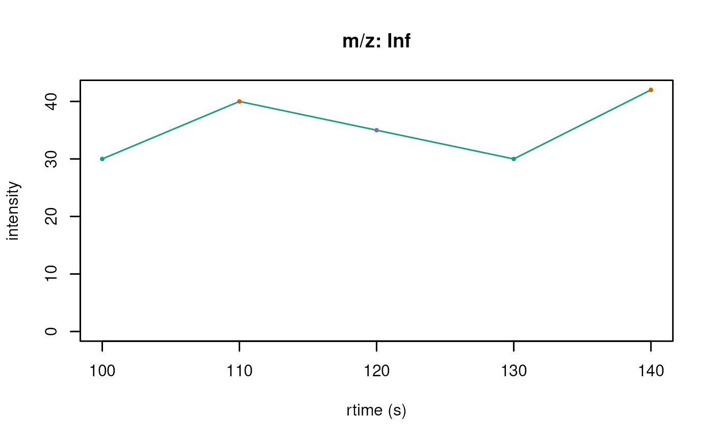
On the overhand if the users wants to easily compare the
chromatograms, the plotChromatogramsOverlay() function can
be used to overlay all chromatograms into one plot.
plotChromatogramsOverlay(chr_s, col = col3)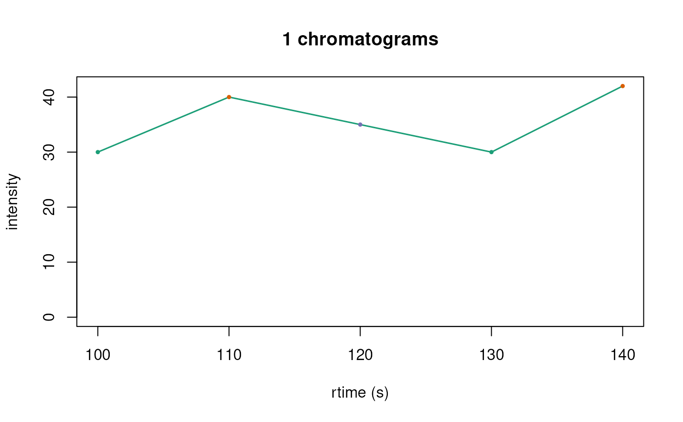
Extracting chromatographic regions of interest
The chromExtract() function allows you to extract
specific regions of interest from a Chromatograms object
based on a peak table. This is particularly useful when you want to
focus on specific retention time windows or m/z ranges that correspond
to detected peaks or features of interest.
Basic extraction by retention time
For backends like ChromBackendMemory and
ChromBackendMzR, you can extract regions based on retention
time ranges:
## Define peaks of interest with retention time windows
peak_table <- data.frame(
    rtMin = c(8, 11),
    rtMax = c(10, 13),
    msLevel = c(2L, 2L),
    chromIndex = c(1L, 2L)
)

## Extract those regions
chr_extracted <- chromExtract(chr, peak_table,
                              by = c("msLevel", "chromIndex"))

chr_extracted
## Chromatographic data (Chromatograms) with 2 chromatograms in a ChromBackendMemory backend:
## chromIndex msLevel mz
## 1 1 2 112.2
## 2 2 2 123.3
## ... 3 more chromatogram variables/columns
## ... 2 peaksData variablesThe resulting Chromatograms object contains only the
data within the specified retention time windows. Note that extra
columns in peak_table are added to the chromatogram
metadata:
chromData(chr_extracted)## msLevel mz chromIndex extra rtMin rtMax collisionEnergy dataOrigin mzMin
## 1 2 112.2 1 extra1 8 10 NA <NA> NA
## 2 2 123.3 2 extra2 11 13 NA <NA> NA
## mzMax precursorMz precursorMzMin precursorMzMax productMz productMzMin
## 1 NA NA NA NA NA NA
## 2 NA NA NA NA NA NA
## productMzMax
## 1 NA
## 2 NAExtraction with m/z filtering (ChromBackendSpectra only)
When using ChromBackendSpectra, you can also filter by
m/z ranges, which is useful for extracting ion chromatograms (EICs) for
specific mass windows:
## Define peak table with both retention time and m/z windows
peak_table_mz <- data.frame(
    rtMin = c(125, 125),
    rtMax = c(180, 180),
    mzMin = c(100, 140),
    mzMax = c(100.5, 140.5),
    msLevel = c(1L, 1L),
    dataOrigin = rep(dataOrigin(chr_s)[1], 2),
    featureID = c("feature_1", "feature_2")
)

## Extract EICs for these features
chr_eics <- chromExtract(chr_s, peak_table_mz,
                        by = c("msLevel", "dataOrigin"))

chr_eics
## Chromatographic data (Chromatograms) with 2 chromatograms in a ChromBackendSpectra backend:
## chromIndex msLevel mz
## 1 NA 1 Inf
## 2 NA 1 Inf
## ... 18 more chromatogram variables/columns
## ... 2 peaksData variables
##
## The Spectra object contains 5 spectraNotice that the custom column featureID from the peak
table is now part of the chromatogram metadata:
chromData(chr_eics)## msLevel rtMin rtMax mzMin mzMax mz dataOrigin chromSpectraIndex chromIndex
## 1 1 125 180 100 100.5 Inf example 1_example NA
## 2 1 125 180 140 140.5 Inf example 1_example NA
## collisionEnergy precursorMz precursorMzMin precursorMzMax productMz
## 1 NA NA NA NA NA
## 2 NA NA NA NA NA
## productMzMin productMzMax rtmin rtmax mzmin mzmax featureID
## 1 NA NA 125 180 100 100.5 feature_1
## 2 NA NA 125 180 100 100.5 feature_2This is particularly useful for linking extracted chromatograms back to feature tables or peak detection results.
Imputing missing values in chromatograms
Real chromatographic data often has gaps or missing intensity values
at certain retention times, which can occur due to instrumental
limitations, data processing artifacts, or sparse sampling. The
imputePeaksData() function provides several methods to
interpolate these missing values, which can improve downstream analysis
and visualization.
Available imputation methods
The package provides four imputation methods:
- “linear”: Linear interpolation between known values. Fast and simple, good for data with regular gaps.
- “spline”: Cubic spline interpolation. Provides smooth curves but may introduce artifacts.
- “gaussian”: Gaussian kernel smoothing. Uses a Gaussian kernel to estimate values based on neighboring points.
- “loess”: Locally weighted scatter plot smoothing. Provides robust smoothing with local polynomial regression.
Extrapolation vs. Interpolation
By default, imputePeaksData() performs only
interpolation (fills gaps between observed values). You can control this
behavior with the extrapolate parameter:
-
extrapolate = FALSE(default): Only interpolation is performed. Leading and trailingNAvalues (outside the range of observed data) remain asNA. -
extrapolate = TRUE: Both interpolation and extrapolation are performed. AllNAvalues are filled.
Example: Imputing an extracted ion chromatogram (EIC)
To demonstrate imputation we first build a small Spectra
object that already contains a few NA intensity values —
mimicking a real-world EIC with gaps — and then extract a chromatogram
from it.
## A small Spectra with some missing intensities at m/z 100
sp_gaps <- Spectra(
    DataFrame(
        rtime      = c(100, 110, 120, 130, 140, 150, 160, 170, 180),
        msLevel    = rep(1L, 9),
        dataOrigin = rep("impute_demo", 9),
        mz = NumericList(100, 100, 100, 100, 100, 100, 100, 100, 100,
                         compress = FALSE),
        intensity = NumericList(50, NA, 120, 200, NA, NA, 80, 30, 10,
                               compress = FALSE)
    ),
    source = MsBackendDataFrame()
)

## Derive a Chromatograms and extract the EIC for m/z ≈ 100
chr_gaps <- Chromatograms(sp_gaps)
eic_table <- data.frame(
    rtMin = 100, rtMax = 180,
    mzMin = 99.5, mzMax = 100.5,
    msLevel = 1L,
    dataOrigin = "impute_demo"
)

chr_eic <- chromExtract(chr_gaps, eic_table,
                        by = c("msLevel", "dataOrigin"))
chr_eic
## Chromatographic data (Chromatograms) with 1 chromatograms in a ChromBackendSpectra backend:
## chromIndex msLevel mz
## 1 NA 1 Inf
## ... 6 more chromatogram variables/columns
## ... 2 peaksData variables
##
## The Spectra object contains 9 spectraNow let’s examine the raw data and apply different imputation methods:
## Create copies for comparison
chr_linear <- imputePeaksData(chr_eic, method = "linear")
chr_spline <- imputePeaksData(chr_eic, method = "spline")
chr_gaussian <- imputePeaksData(chr_eic, method = "gaussian",
                                window = 2, sd = 1)
chr_loess <- imputePeaksData(chr_eic, method = "loess", span = 0.75)

## Plot all methods for comparison
par(mfrow = c(3, 2), mar = c(4, 4, 2, 1))

## Original data
plotChromatograms(chr_eic, main = "Original EIC")

## Linear interpolation
plotChromatograms(chr_linear, main = "Linear Imputation")
## The `peaksData` slot will be modified but the changes will not affect the Spectra object.
## Spline interpolation
plotChromatograms(chr_spline, main = "Spline Imputation")
## The `peaksData` slot will be modified but the changes will not affect the Spectra object.
## Gaussian smoothing
plotChromatograms(chr_gaussian, main = "Gaussian Smoothing (window=2, sd=1)")
## The `peaksData` slot will be modified but the changes will not affect the Spectra object.
## LOESS smoothing
plotChromatograms(chr_loess, main = "LOESS Smoothing (span=0.75)")
## Warning in simpleLoess(y, x, w, span, degree = degree, parametric = parametric,
## : pseudoinverse used at 4## Warning in simpleLoess(y, x, w, span, degree = degree, parametric = parametric,
## : neighborhood radius 3## Warning in simpleLoess(y, x, w, span, degree = degree, parametric = parametric,
## : reciprocal condition number 0## The `peaksData` slot will be modified but the changes will not affect the Spectra object.
Selecting the right imputation method
The choice of imputation method depends on your data characteristics and analysis goals:
- Use “linear” for quick interpolation of small gaps in regularly sampled data.
- Use “spline” for smooth curves when data is fairly regular, but be aware it can overshoot.
- Use “gaussian” for local smoothing that preserves peak shapes while filling gaps.
- Use “loess” when you want robust smoothing that adapts to local data density.
Imputation in lazy evaluation pipelines
For on-disk backends like ChromBackendMzR, imputation is
particularly useful when combined with the lazy evaluation queue. The
imputation function is added to the processing queue and is only applied
when peak data is actually accessed:
## For on-disk backends, add imputation to the lazy queue
chr_mzr_imputed <- imputePeaksData(
  chr_mzr,
  method = "gaussian",
  window = 5,
  sd = 2
)

chr_mzr_imputed
## Chromatographic data (Chromatograms) with 138 chromatograms in a ChromBackendMemory backend:
## chromIndex msLevel mz
## 1 1 NA NA
## 2 2 NA NA
## 3 3 NA NA
## 4 4 NA NA
## 5 5 NA NA
## 6 6 NA NA
## ... 6 more chromatogram variables/columns
## ... 2 peaksData variables
## Lazy evaluation queue: 1 processing step(s)
## Processing:
## Switch backend from ChromBackendMzR to ChromBackendMemory [Sat May 23 14:11:37 2026]
## Impute: replace missing peaks data using the 'gaussian' method [Sat May 23 14:11:39 2026]The imputation is not performed immediately.
Instead, it’s stored in the processing queue. When you call
peaksData() on the object, the raw data is read from the
file and then imputation is applied on-the-fly:
## This reads from disk and applies imputation in one step
peak_data <- peaksData(chr_mzr_imputed[1])
This approach is highly efficient for large datasets because:
- Data is only read from disk when needed
- Imputation is applied on-the-fly during data access
- No temporary files are created
- Memory usage remains minimal
You can verify the processing queue contains your imputation step:
length(chr_mzr_imputed@processingQueue)## [1] 1And if you want to make the imputation permanent (for in-memory
backends), use applyProcessing():
## For in-memory backends, you can persist the imputation
chr_in_memory <- setBackend(chr_mzr_imputed, ChromBackendMemory())
chr_in_memory <- applyProcessing(chr_in_memory)

# Now imputation is permanently applied
length(chr_in_memory@processingQueue)
## [1] 0Comparing chromatograms
The compareChromatograms() function computes pairwise
similarity between chromatograms in two steps. First, a mapping function
(MAPFUN, default matchRtime()) aligns two
chromatograms onto a common retention-time grid by linear interpolation,
returning aligned intensity vectors for each. Then, a scoring function
(FUN, default cor(), i.e. Pearson correlation)
computes a similarity value from those vectors. Additional arguments
such as method = "spearman" can be passed via
... to the scoring function, and a fully custom
FUN or MAPFUN can be supplied.
The result is always a 3-dimensional numeric array of dimensions
n × m × 2. Layer [, , "score"] contains pairwise
similarity scores; layer [, , "n_peaks"] contains the
number of overlapping retention-time points used for each comparison.
The minPeaks parameter (default 4) sets the
minimum number of overlapping points required to compute a score — pairs
below this threshold return NA in the score layer while the
actual overlap count is still recorded in n_peaks. This
avoids unreliable scores from very sparse overlaps and skips the
FUN computation entirely for those pairs. Use
minPeaks = 2L to compute a score whenever two or more
points overlap.
Comparing chromatograms within a single object
When called with a single Chromatograms object,
compareChromatograms() computes all pairwise similarities
and returns a symmetric n × n × 2 array.
Let’s pick a subset of the MRM chromatograms we loaded earlier:
## Pick 8 MRM chromatograms, skipping the first (a TIC with no m/z info)
chr_sub <- chr_mzr[2:9]

cor_arr <- compareChromatograms(chr_sub)
cor_arr[, , "score"]   ## similarity scores
## [,1] [,2] [,3] [,4] [,5] [,6] [,7]
## [1,] 1.00000000 0.95316189 0.8226159 0.8006447 0.9070273 0.04796832 0.9008680
## [2,] 0.95316189 1.00000000 0.9223071 0.9055515 0.9634465 0.09180481 0.9745576
## [3,] 0.82261589 0.92230714 1.0000000 0.9901850 0.8994321 0.11162745 0.9482596
## [4,] 0.80064470 0.90555155 0.9901850 1.0000000 0.8718728 0.11893327 0.9276409
## [5,] 0.90702731 0.96344649 0.8994321 0.8718728 1.0000000 0.13258748 0.9780192
## [6,] 0.04796832 0.09180481 0.1116274 0.1189333 0.1325875 1.00000000 0.1300610
## [7,] 0.90086802 0.97455760 0.9482596 0.9276409 0.9780192 0.13006103 1.0000000
## [8,] 0.89938262 0.97415279 0.9452776 0.9241078 0.9782780 0.13103957 0.9995715
## [,8]
## [1,] 0.8993826
## [2,] 0.9741528
## [3,] 0.9452776
## [4,] 0.9241078
## [5,] 0.9782780
## [6,] 0.1310396
## [7,] 0.9995715
## [8,] 1.0000000
cor_arr[, , "n_peaks"] ## number of overlapping RT points per pair## [,1] [,2] [,3] [,4] [,5] [,6] [,7] [,8]
## [1,] 962 961 444 444 444 444 444 444
## [2,] 961 962 444 444 444 444 444 444
## [3,] 444 444 523 522 520 520 522 522
## [4,] 444 444 522 523 520 520 522 522
## [5,] 444 444 520 520 521 520 521 521
## [6,] 444 444 520 520 520 521 521 521
## [7,] 444 444 522 522 521 521 523 522
## [8,] 444 444 522 522 521 521 522 523
## Use a chromData column as row/column labels
cor_arr_labeled <- compareChromatograms(chr_sub, labelsColumn = "chromIndex")
cor_arr_labeled[, , "score"]
## 2 3 4 5 6 7 8
## 2 1.00000000 0.95316189 0.8226159 0.8006447 0.9070273 0.04796832 0.9008680
## 3 0.95316189 1.00000000 0.9223071 0.9055515 0.9634465 0.09180481 0.9745576
## 4 0.82261589 0.92230714 1.0000000 0.9901850 0.8994321 0.11162745 0.9482596
## 5 0.80064470 0.90555155 0.9901850 1.0000000 0.8718728 0.11893327 0.9276409
## 6 0.90702731 0.96344649 0.8994321 0.8718728 1.0000000 0.13258748 0.9780192
## 7 0.04796832 0.09180481 0.1116274 0.1189333 0.1325875 1.00000000 0.1300610
## 8 0.90086802 0.97455760 0.9482596 0.9276409 0.9780192 0.13006103 1.0000000
## 9 0.89938262 0.97415279 0.9452776 0.9241078 0.9782780 0.13103957 0.9995715
## 9
## 2 0.8993826
## 3 0.9741528
## 4 0.9452776
## 5 0.9241078
## 6 0.9782780
## 7 0.1310396
## 8 0.9995715
## 9 1.0000000We can visualise the score layer as a heatmap, labelling rows and
columns with the MRM precursor → product m/z transitions stored in
chromData():
library(pheatmap)
## Label rows/columns with precursor → product m/z transitions
mz_labels <- paste0(round(chromData(chr_sub)$precursorMz, 1), " → ",
                     round(chromData(chr_sub)$productMz, 1))
score_mat <- cor_arr[, , "score"]
rownames(score_mat) <- colnames(score_mat) <- mz_labels
pheatmap(score_mat, main = "Pairwise Pearson correlation",
         color = hcl.colors(30, palette = "RdYlBu", rev = TRUE))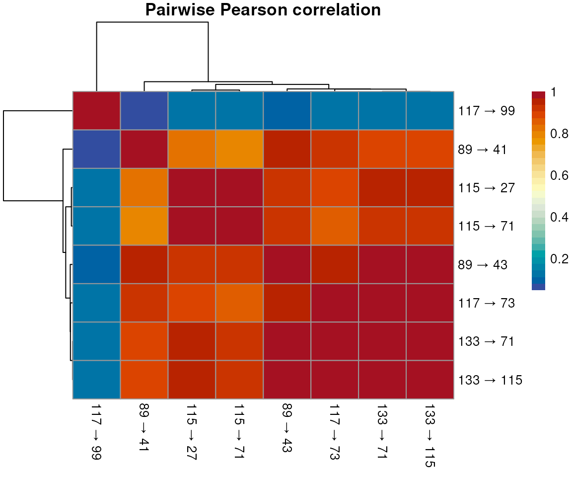
A custom similarity function can be passed via FUN. For
example, cosine similarity, useful for checking co-elution regardless of
absolute intensity differences:
cosine <- function(x, y) {
    sum(x * y) / (sqrt(sum(x^2)) * sqrt(sum(y^2)))
}

cos_arr <- compareChromatograms(chr_sub, FUN = cosine)
cos_arr[, , "score"]
## [,1] [,2] [,3] [,4] [,5] [,6] [,7]
## [1,] 1.0000000 0.8627648 0.9644232 0.4951596 0.4579415 0.9727773 0.3352872
## [2,] 0.8627648 1.0000000 0.9897048 0.7092739 0.6930469 0.9145884 0.5958371
## [3,] 0.9644232 0.9897048 1.0000000 0.6862612 0.6431259 0.9384094 0.5222776
## [4,] 0.4951596 0.7092739 0.6862612 1.0000000 0.8948345 0.4501788 0.9186125
## [5,] 0.4579415 0.6930469 0.6431259 0.8948345 1.0000000 0.4307590 0.9664627
## [6,] 0.9727773 0.9145884 0.9384094 0.4501788 0.4307590 1.0000000 0.2780748
## [7,] 0.3352872 0.5958371 0.5222776 0.9186125 0.9664627 0.2780748 1.0000000
## [8,] 0.3218180 0.5843252 0.5085146 0.9122729 0.9639578 0.2640564 0.9994836
## [,8]
## [1,] 0.3218180
## [2,] 0.5843252
## [3,] 0.5085146
## [4,] 0.9122729
## [5,] 0.9639578
## [6,] 0.2640564
## [7,] 0.9994836
## [8,] 1.0000000The n_peaks layer is useful even when
minPeaks blocks a score: it shows how many RT points
overlapped, letting you distinguish no overlap at all
(n_peaks = 0) from some overlap but below the
threshold (n_peaks > 0 but
score = NA):
## Require at least 10 overlapping RT points to compute a score
cor_strict <- compareChromatograms(chr_sub, minPeaks = 10L)
cor_strict[, , "score"]   ## NAs for pairs with < 10 common RT points
## [,1] [,2] [,3] [,4] [,5] [,6] [,7]
## [1,] 1.00000000 0.95316189 0.8226159 0.8006447 0.9070273 0.04796832 0.9008680
## [2,] 0.95316189 1.00000000 0.9223071 0.9055515 0.9634465 0.09180481 0.9745576
## [3,] 0.82261589 0.92230714 1.0000000 0.9901850 0.8994321 0.11162745 0.9482596
## [4,] 0.80064470 0.90555155 0.9901850 1.0000000 0.8718728 0.11893327 0.9276409
## [5,] 0.90702731 0.96344649 0.8994321 0.8718728 1.0000000 0.13258748 0.9780192
## [6,] 0.04796832 0.09180481 0.1116274 0.1189333 0.1325875 1.00000000 0.1300610
## [7,] 0.90086802 0.97455760 0.9482596 0.9276409 0.9780192 0.13006103 1.0000000
## [8,] 0.89938262 0.97415279 0.9452776 0.9241078 0.9782780 0.13103957 0.9995715
## [,8]
## [1,] 0.8993826
## [2,] 0.9741528
## [3,] 0.9452776
## [4,] 0.9241078
## [5,] 0.9782780
## [6,] 0.1310396
## [7,] 0.9995715
## [8,] 1.0000000
cor_strict[, , "n_peaks"] ## actual overlap counts are always recorded## [,1] [,2] [,3] [,4] [,5] [,6] [,7] [,8]
## [1,] 962 961 444 444 444 444 444 444
## [2,] 961 962 444 444 444 444 444 444
## [3,] 444 444 523 522 520 520 522 522
## [4,] 444 444 522 523 520 520 522 522
## [5,] 444 444 520 520 521 520 521 521
## [6,] 444 444 520 520 520 521 521 521
## [7,] 444 444 522 522 521 521 523 522
## [8,] 444 444 522 522 521 521 522 523Comparing two Chromatograms objects
When called with two Chromatograms objects,
compareChromatograms(x, y) returns an n × m × 2
array with similarities between each chromatogram in x
(rows) and each in y (columns).
## Compare the first 4 chromatograms against the last 4
res <- compareChromatograms(chr_sub[1:4], chr_sub[5:8])
res[, , "score"]
## [,1] [,2] [,3] [,4]
## [1,] 0.9070273 0.04796832 0.9008680 0.8993826
## [2,] 0.9634465 0.09180481 0.9745576 0.9741528
## [3,] 0.8994321 0.11162745 0.9482596 0.9452776
## [4,] 0.8718728 0.11893327 0.9276409 0.9241078Comparing groups of chromatograms
To compare chromatograms within separate groups (e.g. per
dataOrigin), split the object first and apply
compareChromatograms() to each subset:
Session information
## R version 4.6.0 (2026-04-24)
## Platform: x86_64-pc-linux-gnu
## Running under: Ubuntu 24.04.4 LTS
##
## Matrix products: default
## BLAS:   /usr/lib/x86_64-linux-gnu/openblas-pthread/libblas.so.3
## LAPACK: /usr/lib/x86_64-linux-gnu/openblas-pthread/libopenblasp-r0.3.26.so;  LAPACK version 3.12.0
##
## locale:
##  [1] LC_CTYPE=en_US.UTF-8       LC_NUMERIC=C
##  [3] LC_TIME=en_US.UTF-8        LC_COLLATE=en_US.UTF-8
##  [5] LC_MONETARY=en_US.UTF-8    LC_MESSAGES=en_US.UTF-8
##  [7] LC_PAPER=en_US.UTF-8       LC_NAME=C
##  [9] LC_ADDRESS=C               LC_TELEPHONE=C
## [11] LC_MEASUREMENT=en_US.UTF-8 LC_IDENTIFICATION=C
##
## time zone: UTC
## tzcode source: system (glibc)
##
## attached base packages:
## [1] stats4    stats     graphics  grDevices utils     datasets  methods
## [8] base
##
## other attached packages:
##  [1] pheatmap_1.0.13     RColorBrewer_1.1-3  IRanges_2.47.1
##  [4] Spectra_1.23.0      S4Vectors_0.51.2    BiocGenerics_0.59.2
##  [7] generics_0.1.4      Chromatograms_1.3.0 ProtGenerics_1.45.0
## [10] BiocParallel_1.47.0 BiocStyle_2.41.0
##
## loaded via a namespace (and not attached):
##  [1] sass_0.4.10            MsCoreUtils_1.25.4     digest_0.6.39
##  [4] evaluate_1.0.5         grid_4.6.0             bookdown_0.46
##  [7] fastmap_1.2.0          jsonlite_2.0.0         mzR_2.47.0
## [10] BiocManager_1.30.27    scales_1.4.0           codetools_0.2-20
## [13] textshaping_1.0.5      jquerylib_0.1.4        cli_3.6.6
## [16] rlang_1.2.0            Biobase_2.73.1         cachem_1.1.0
## [19] yaml_2.3.12            otel_0.2.0             tools_4.6.0
## [22] parallel_4.6.0         ncdf4_1.24             R6_2.6.1
## [25] lifecycle_1.0.5        fs_2.1.0               htmlwidgets_1.6.4
## [28] clue_0.3-68            MASS_7.3-65            ragg_1.5.2
## [31] cluster_2.1.8.2        desc_1.4.3             pkgdown_2.2.0.9000
## [34] bslib_0.11.0           gtable_0.3.6           data.table_1.18.4
## [37] glue_1.8.1             Rcpp_1.1.1-1.1         systemfonts_1.3.2
## [40] xfun_0.57              knitr_1.51             farver_2.1.2
## [43] htmltools_0.5.9        rmarkdown_2.31         compiler_4.6.0
## [46] MetaboCoreUtils_1.21.1