Description and Usage of MsBackendMassbank
Source:vignettes/MsBackendMassbank.Rmd
MsBackendMassbank.RmdPackage: MsBackendMassbank
Authors: RforMassSpectrometry Package Maintainer [cre],
Michael Witting [aut] (ORCID: https://orcid.org/0000-0002-1462-4426), Johannes Rainer
[aut] (ORCID: https://orcid.org/0000-0002-6977-7147), Michael Stravs
[ctb]
Compiled: Wed Mar 18 15:05:56 2026
Introduction
The Spectra package provides a central infrastructure for the handling of mass spectrometry (MS) data. The package supports interchangeable use of different backends to import MS data from a variety of sources (such as mzML files). The MsBackendMassbank package allows import and handling MS/MS spectrum data from Massbank. This vignette illustrates the usage of the MsBackendMassbank package to include MassBank data into MS data analysis workflow with the Spectra package in R.
Installation
The package can be installed with the BiocManager package.
To install BiocManager use
install.packages("BiocManager") and, after that,
BiocManager::install("MsBackendMassbank") to install this
package.
Importing MS/MS data from MassBank files
MassBank is an open-source, community managed spectral library. All
data is available in the MassBank GitHub
page, where releases are provided (which are also shared through Zenodo,
with their own release-specific DOI). MassBank stores and shares data
through individual text files (one file per spectrum) in a specific
MassBank format. These files can be imported (as well as exported) with
the MsBackendMassbank class of the MsBackendMassbank
package.
In our example below we load the required libraries and define the (full) paths to example MassBank files available in this package.
library(Spectra)
library(MsBackendMassbank)
fls <- dir(system.file("extdata", package = "MsBackendMassbank"),
           full.names = TRUE, pattern = "txt$")
fls
## [1] "/__w/_temp/Library/MsBackendMassbank/extdata/BSU00001.txt"
## [2] "/__w/_temp/Library/MsBackendMassbank/extdata/MassBankRecords.txt"
## [3] "/__w/_temp/Library/MsBackendMassbank/extdata/MSBNK-UFZ-UA000101.txt"
## [4] "/__w/_temp/Library/MsBackendMassbank/extdata/multi_precursor_mz.txt"
## [5] "/__w/_temp/Library/MsBackendMassbank/extdata/RP000501_mod.txt"
## [6] "/__w/_temp/Library/MsBackendMassbank/extdata/RP000501.txt"
## [7] "/__w/_temp/Library/MsBackendMassbank/extdata/RP000502.txt"
## [8] "/__w/_temp/Library/MsBackendMassbank/extdata/RP000503.txt"
## [9] "/__w/_temp/Library/MsBackendMassbank/extdata/RP000511.txt"
## [10] "/__w/_temp/Library/MsBackendMassbank/extdata/RP000512.txt"
## [11] "/__w/_temp/Library/MsBackendMassbank/extdata/RP000513.txt"MS data can be accessed and analyzed through Spectra
objects. Below we create a Spectra object with the data
from these MassBank files. To this end we provide the file names and
specify to use a MsBackendMassbank() backend as
source to enable data import.
sps <- Spectra(fls,
               source = MsBackendMassbank(),
               backend = MsBackendDataFrame(),
               nonStop = TRUE)
With that we have now full access to all imported spectra variables (spectrum metadata fields) that we list below.
spectraVariables(sps)## [1] "msLevel" "rtime"
## [3] "acquisitionNum" "scanIndex"
## [5] "dataStorage" "dataOrigin"
## [7] "centroided" "smoothed"
## [9] "polarity" "precScanNum"
## [11] "precursorMz" "precursorIntensity"
## [13] "precursorCharge" "collisionEnergy"
## [15] "isolationWindowLowerMz" "isolationWindowTargetMz"
## [17] "isolationWindowUpperMz" "acquistionNum"
## [19] "accession" "name"
## [21] "smiles" "exactmass"
## [23] "formula" "inchi"
## [25] "cas" "inchikey"
## [27] "adduct" "splash"
## [29] "title"We can for example access the compound name for each spectrum.
sps$name## [[1]]
## [1] "Veratramine"
## [2] "(3beta,23R)-14,15,16,17-Tetradehydroveratraman-3,23-diol"
##
## [[2]]
## [1] "L-Tryptophan"
## [2] "(2S)-2-amino-3-(1H-indol-3-yl)propanoic acid"
##
## [[3]]
## [1] "L-Tryptophan"
## [2] "(2S)-2-amino-3-(1H-indol-3-yl)propanoic acid"
##
## [[4]]
## [1] "L-Tryptophan"
## [2] "(2S)-2-amino-3-(1H-indol-3-yl)propanoic acid"
##
## [[5]]
## [1] "Carbazole" "9H-carbazole"
##
## [[6]]
## [1] "L-Tryptophan"
## [2] "(2S)-2-amino-3-(1H-indol-3-yl)propanoic acid"
##
## [[7]]
## [1] "L-Tryptophan"
## [2] "(2S)-2-amino-3-(1H-indol-3-yl)propanoic acid"
##
## [[8]]
## [1] "L-Tryptophan"
## [2] "(2S)-2-amino-3-(1H-indol-3-yl)propanoic acid"
##
## [[9]]
## [1] "L-Tryptophan"
## [2] "(2S)-2-amino-3-(1H-indol-3-yl)propanoic acid"
##
## [[10]]
## [1] "L-Tryptophan"
##
## [[11]]
## [1] "L-Tryptophan"
## [2] "(2S)-2-amino-3-(1H-indol-3-yl)propanoic acid"
##
## [[12]]
## [1] "L-Tryptophan"
## [2] "(2S)-2-amino-3-(1H-indol-3-yl)propanoic acid"MassBank allows defining more than one name for a compound and the
result is thus returned as a list with all provided names
and aliases per spectrum.
By default only some of the metadata fields available in the MassBank
files are imported. Through the metaBlocks parameter it is
possible to enable also import of additional blocks of metadata fields
(which results however in a slower data import). Below we use the
metaDataBlocks() function to configure the blocks to
import. We select to import the $AC and $MS
fields:
#' define the metadata blocks to import
mdb <- metaDataBlocks(ac = TRUE, ms = TRUE)

#' import the data
sps <- Spectra(fls,
               source = MsBackendMassbank(),
               metaBlock = mdb)
A larger number of spectra variables is now available:
spectraVariables(sps)## [1] "msLevel" "rtime"
## [3] "acquisitionNum" "scanIndex"
## [5] "dataStorage" "dataOrigin"
## [7] "centroided" "smoothed"
## [9] "polarity" "precScanNum"
## [11] "precursorMz" "precursorIntensity"
## [13] "precursorCharge" "collisionEnergy"
## [15] "isolationWindowLowerMz" "isolationWindowTargetMz"
## [17] "isolationWindowUpperMz" "acquistionNum"
## [19] "accession" "name"
## [21] "smiles" "exactmass"
## [23] "formula" "inchi"
## [25] "cas" "inchikey"
## [27] "adduct" "splash"
## [29] "title" "instrument"
## [31] "instrument_type" "ms_ms_type"
## [33] "ms_cap_voltage" "ms_col_gas"
## [35] "ms_desolv_gas_flow" "ms_desolv_temp"
## [37] "ms_frag_mode" "ms_ionization"
## [39] "ms_ionization_energy" "ms_ionization_voltage"
## [41] "ms_laser" "ms_matrix"
## [43] "ms_mass_accuracy" "ms_mass_range"
## [45] "ms_reagent_gas" "ms_resolution"
## [47] "ms_scan_setting" "ms_source_temp"
## [49] "ms_kinetic_energy" "ms_electron_current"
## [51] "ms_reaction_time" "chrom_carrier_gas"
## [53] "chrom_column" "chrom_column_temp"
## [55] "chrom_column_temp_gradient" "chrom_flow_gradient"
## [57] "chrom_flow_rate" "chrom_inj_temp"
## [59] "chrom_inj_temp_gradient" "chrom_rti_kovats"
## [61] "chrom_rti_lee" "chrom_rti_naps"
## [63] "chrom_rti_uoa" "chrom_rti_uoa_pred"
## [65] "chrom_rt" "chrom_rt_uoa_pred"
## [67] "chrom_solvent" "chrom_transfer_temp"
## [69] "ims_instrument_type" "ims_drift_gas"
## [71] "ims_drift_time" "ims_ccs"
## [73] "general_conc" "focus_base_peak"
## [75] "focus_derivative_form" "focus_derivative_mass"
## [77] "focus_derivative_type" "focus_ion_type"
## [79] "data_processing_comment" "data_processing_deprofile"
## [81] "data_processing_find_peak" "data_processing_reanalyze"
## [83] "data_processing_recalibrate" "data_processing_whole"For some of these, however, no information might be provided. To
remove spectra variables that have only missing values for
all spectra, we can use the
dropNaSpectraVariables() function:
sps <- dropNaSpectraVariables(sps)
spectraVariables(sps)
## [1] "msLevel" "rtime"
## [3] "acquisitionNum" "scanIndex"
## [5] "dataStorage" "dataOrigin"
## [7] "centroided" "smoothed"
## [9] "polarity" "precScanNum"
## [11] "precursorMz" "precursorIntensity"
## [13] "precursorCharge" "collisionEnergy"
## [15] "isolationWindowLowerMz" "isolationWindowTargetMz"
## [17] "isolationWindowUpperMz" "acquistionNum"
## [19] "accession" "name"
## [21] "smiles" "exactmass"
## [23] "formula" "inchi"
## [25] "cas" "inchikey"
## [27] "adduct" "splash"
## [29] "title" "instrument"
## [31] "instrument_type" "ms_ms_type"
## [33] "ms_frag_mode" "ms_ionization"
## [35] "ms_resolution" "chrom_column"
## [37] "chrom_flow_gradient" "chrom_flow_rate"
## [39] "chrom_rt" "chrom_solvent"
## [41] "focus_base_peak" "data_processing_reanalyze"
## [43] "data_processing_recalibrate" "data_processing_whole"When importing a large number of MassBank files, setting
nonStop = TRUE prevents the call to stop whenever
problematic MassBank files are encountered.
Accessing the MassBank MySQL database
An alternative to the import of the MassBank data from individual text files (which can take a considerable amount of time) is to directly access the MS/MS data in the MassBank MySQL database. For demonstration purposes we are using here a tiny subset of the MassBank data which is stored as a SQLite database within this package.
Pre-requisites
At present it is not possible to directly connect to the main
MassBank production MySQL server, thus, to use the
MsBackendMassbankSql backend it is required to install the
database locally. The MySQL database dump for each MassBank release can
be downloaded the MassBank GitHub repository (for most releases). This
dump could be imported to a local MySQL server.
Direct access to the MassBank database
To use the MsBackendMassbankSql it is required to first
connect to a MassBank database. Below we show the R code which
could be used for that - but the actual settings (user name, password,
database name, or host) will depend on where and how the MassBank
database was installed.
library(RMariaDB)
con <- dbConnect(MariaDB(), host = "localhost", user = "massbank",
                 dbname = "MassBank")
To illustrate the general functionality of this backend we use a tiny subset of the MassBank (release 2020.10) which is provided as an small SQLite database within this package. Below we connect to this database.
library(RSQLite)
con <- dbConnect(SQLite(), system.file("sql", "minimassbank.sqlite",
                                       package = "MsBackendMassbank"))
We next initialize the MsBackendMassbankSql
backend which supports direct access to the MassBank in a SQL database
and create a Spectra object from that.
mb <- Spectra(con, source = MsBackendMassbankSql())
mb
## MSn data (Spectra) with 70 spectra in a MsBackendMassbankSql backend:
## msLevel precursorMz polarity
## <integer> <numeric> <integer>
## 1 2 506 0
## 2 NA NA 1
## 3 NA NA 0
## 4 NA NA 1
## 5 NA NA 0
## ... ... ... ...
## 66 2 185.028 0
## 67 2 455.290 1
## 68 2 253.051 0
## 69 2 358.238 1
## 70 2 256.170 1
## ... 41 more variables/columns.
## Use 'spectraVariables' to list all of them.We can now use this Spectra object to access and use the
MassBank data for our analysis. Note that the Spectra
object itself does not contain any data from MassBank. Any data will be
fetched on demand from the database backend.
To get a listing of all available annotations for each spectrum (the
so-called spectra variables) we can use the
spectraVariables() function.
spectraVariables(mb)## [1] "msLevel" "rtime"
## [3] "acquisitionNum" "scanIndex"
## [5] "dataStorage" "dataOrigin"
## [7] "centroided" "smoothed"
## [9] "polarity" "precScanNum"
## [11] "precursorMz" "precursorIntensity"
## [13] "precursorCharge" "collisionEnergy"
## [15] "isolationWindowLowerMz" "isolationWindowTargetMz"
## [17] "isolationWindowUpperMz" "spectrum_id"
## [19] "spectrum_name" "date"
## [21] "authors" "license"
## [23] "copyright" "publication"
## [25] "splash" "compound_id"
## [27] "adduct" "ionization"
## [29] "ionization_voltage" "fragmentation_mode"
## [31] "instrument" "instrument_type"
## [33] "formula" "exactmass"
## [35] "smiles" "inchi"
## [37] "inchikey" "cas"
## [39] "pubchem" "synonym"
## [41] "precursor_mz_text" "compound_name"Through the MsBackendMassbankSql we can thus access
spectra information as well as its annotation.
We can access core spectra variables, such as the MS level
with the corresponding function msLevel().
## [1] 2 NA NA NA NA 2Spectra variables can also be accessed with $ and the
name of the variable. Thus, MS levels can also be accessed with
$msLevel:
head(mb$msLevel)## [1] 2 NA NA NA NA 2In addition to spectra variables, we can also get the actual peaks
(i.e. m/z and intensity values) with the mz() and
intensity() functions:
mz(mb)## NumericList of length 70
## [[1]] 146.760803 158.863541 174.988785 ... 470.057434 487.989319 585.88446
## [[2]] 22.99 23.07 23.19 38.98 53.15 60.08 ... 391.18 413.22 414.22 429.16 495.2
## [[3]] 108.099566 152.005378 153.01824 ... 341.031964 409.06729 499.103447
## [[4]] 137.0227 138.025605 139.034602 ... 304.271886 316.303106 352.234228
## [[5]] 112.977759 205.053323 208.041128 ... 449.137152 671.1778 673.200866
## [[6]] 78.893929 183.011719 193.957916 ... 328.091949 408.010193 426.021942
## [[7]] 167.03389 168.040758 333.079965 ... 357.073039 365.040698 373.073473
## [[8]] 195.09167 196.095033
## [[9]] 108.096149 152.004656 153.01824 ... 359.997563 409.065314 491.043775
## [[10]] 1278.12 1279.11 1279.18 1306.21 ... 2064.29 2091.32 2092.3 2136.33
## ...
## <60 more elements>Note that not all spectra from the database were generated using the same instrumentation. Below we list the number of spectra for each type of instrument.
table(mb$instrument_type)##
## LC-ESI-ITFT LC-ESI-QFT MALDI-TOF
## 3 50 17We next subset the data to all spectra from ions generated by electro spray ionization (ESI).
mb <- mb[mb$ionization == "ESI"]
length(mb)
## [1] 50As a simple example to illustrate the Spectra
functionality we next calculate spectra similarity between one spectrum
against all other spectra in the database. To this end we use the
compareSpectra() function with the normalized dot product
as similarity function and allowing 20 ppm difference in m/z between
matching peaks
library(MsCoreUtils)
sims <- compareSpectra(mb[11], mb[-11], FUN = ndotproduct, ppm = 40)
max(sims)
## [1] 0.7507467We plot next a mirror plot for the two best matching spectra.
plotSpectraMirror(mb[11], mb[(which.max(sims) + 1)], ppm = 40)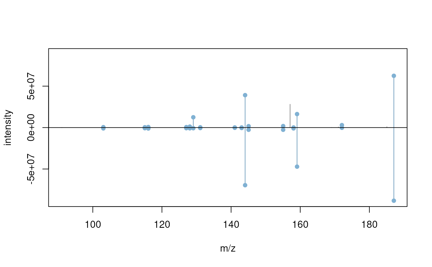
We can also retrieve the compound information for these two
best matching spectra. Note that this compounds() function
works only with the MsBackendMassbankSql backend as it
retrieves the corresponding information from the database’s compound
annotation table.
## DataFrame with 2 rows and 10 columns
##   compound_id     formula exactmass                 smiles
##     <integer> <character> <numeric>            <character>
## 1          31    C12H10O2   186.068 COC1=C(C=O)C2=CC=CC=..
## 2          45    C12H10O2   186.068 COC1=CC=C(C=O)C2=CC=..
##                    inchi               inchikey         cas     pubchem
##              <character>            <character> <character> <character>
## 1 InChI=1S/C12H10O2/c1.. YIQGLTKAOHRZOL-UHFFF..   1/12/5392   CID:79352
## 2 InChI=1S/C12H10O2/c1.. MVXMNHYVCLMLDD-UHFFF..  15971-29-6   CID:85217
##                                         synonym                   name
##                                 <CharacterList>            <character>
## 1 2-Methoxy-1-naphthal..,2-methoxynaphthalene.. 2-Methoxy-1-naphthal..
## 2 4-Methoxy-1-Naphthal..,4-methoxynaphthalene.. 4-Methoxy-1-Naphthal..
Note that the MsBackendMassbankSql backend does not
support parallel processing because the database connection within the
backend can not be shared across parallel processes. Any function on a
Spectra object that uses a
MsBackendMassbankSql will thus (silently) disable any
parallel processing, even if the user might have passed one along to the
function using the BPPARAM parameter. In general, the
backendBpparam() function can be used on any
Spectra object to test whether its backend supports the
provided parallel processing setup (which might be helpful for
developers).
Session information
## R Under development (unstable) (2026-03-15 r89629)
## Platform: x86_64-pc-linux-gnu
## Running under: Ubuntu 24.04.4 LTS
##
## Matrix products: default
## BLAS:   /usr/lib/x86_64-linux-gnu/openblas-pthread/libblas.so.3
## LAPACK: /usr/lib/x86_64-linux-gnu/openblas-pthread/libopenblasp-r0.3.26.so;  LAPACK version 3.12.0
##
## locale:
##  [1] LC_CTYPE=en_US.UTF-8       LC_NUMERIC=C
##  [3] LC_TIME=en_US.UTF-8        LC_COLLATE=en_US.UTF-8
##  [5] LC_MONETARY=en_US.UTF-8    LC_MESSAGES=en_US.UTF-8
##  [7] LC_PAPER=en_US.UTF-8       LC_NAME=C
##  [9] LC_ADDRESS=C               LC_TELEPHONE=C
## [11] LC_MEASUREMENT=en_US.UTF-8 LC_IDENTIFICATION=C
##
## time zone: UTC
## tzcode source: system (glibc)
##
## attached base packages:
## [1] stats4    stats     graphics  grDevices utils     datasets  methods
## [8] base
##
## other attached packages:
## [1] MsCoreUtils_1.23.6       RSQLite_2.4.6            MsBackendMassbank_1.19.3
## [4] Spectra_1.21.5           BiocParallel_1.45.0      S4Vectors_0.49.0
## [7] BiocGenerics_0.57.0      generics_0.1.4           BiocStyle_2.39.0
##
## loaded via a namespace (and not attached):
##  [1] bit_4.6.0              jsonlite_2.0.0         compiler_4.6.0
##  [4] BiocManager_1.30.27    blob_1.3.0             parallel_4.6.0
##  [7] cluster_2.1.8.2        jquerylib_0.1.4        systemfonts_1.3.2
## [10] IRanges_2.45.0         textshaping_1.0.5      yaml_2.3.12
## [13] fastmap_1.2.0          R6_2.6.1               ProtGenerics_1.39.2
## [16] knitr_1.51             htmlwidgets_1.6.4      MASS_7.3-65
## [19] bookdown_0.46          desc_1.4.3             DBI_1.3.0
## [22] bslib_0.10.0           rlang_1.1.7            cachem_1.1.0
## [25] xfun_0.56              fs_1.6.7               sass_0.4.10
## [28] bit64_4.6.0-1          otel_0.2.0             memoise_2.0.1
## [31] cli_3.6.5              pkgdown_2.2.0.9000     digest_0.6.39
## [34] MetaboCoreUtils_1.19.2 lifecycle_1.0.5        clue_0.3-67
## [37] vctrs_0.7.1            data.table_1.18.2.1    evaluate_1.0.5
## [40] codetools_0.2-20       ragg_1.5.1             rmarkdown_2.30
## [43] pkgconfig_2.0.3        tools_4.6.0            htmltools_0.5.9