processQFeatures App

Léopold Guyot

Loïc Guille

22 May 2026

Start the app

Parameters of the Shiny application:

• qfeatures: a QFeatures object. This can be either a path to an RDS file or a QFeatures object already loaded in your R session.

• prefilledSteps (optional): defines the different steps of the workflow used to analyse the QFeatures object. Accepted values are sampleFiltering, featureFiltering, normalisation, missingValuesFeatures, missingValuesSamples, zeroToNA, logTransform, imputation, aggregation, and join. The suggested workflow set as the default value is sampleFiltering, featureFiltering, missingValuesFeatures, missingValuesSamples, normalisation, aggregation, join, and aggregation.

• initialSets (optional): sets to use for the analysis of the QFeatures object. The default is seq_along(qfeatures).

Workflow configuration

A predefined workflow is defined by default with the argument prefilledSteps. If prefilledSteps was modified when the application was launched, this change will be taken into account.

The page contains a brief explanation of each step. To modify the workflow, drag and drop the different steps to be executed on the QFeatures object. Once the workflow is configured, click on Confirm Current Workflow.

If the default workflow is the one you want to use, or if you have already specified the desired workflow in the prefilledSteps parameter, simply click on Step 1.

Sample/Feature Filtering

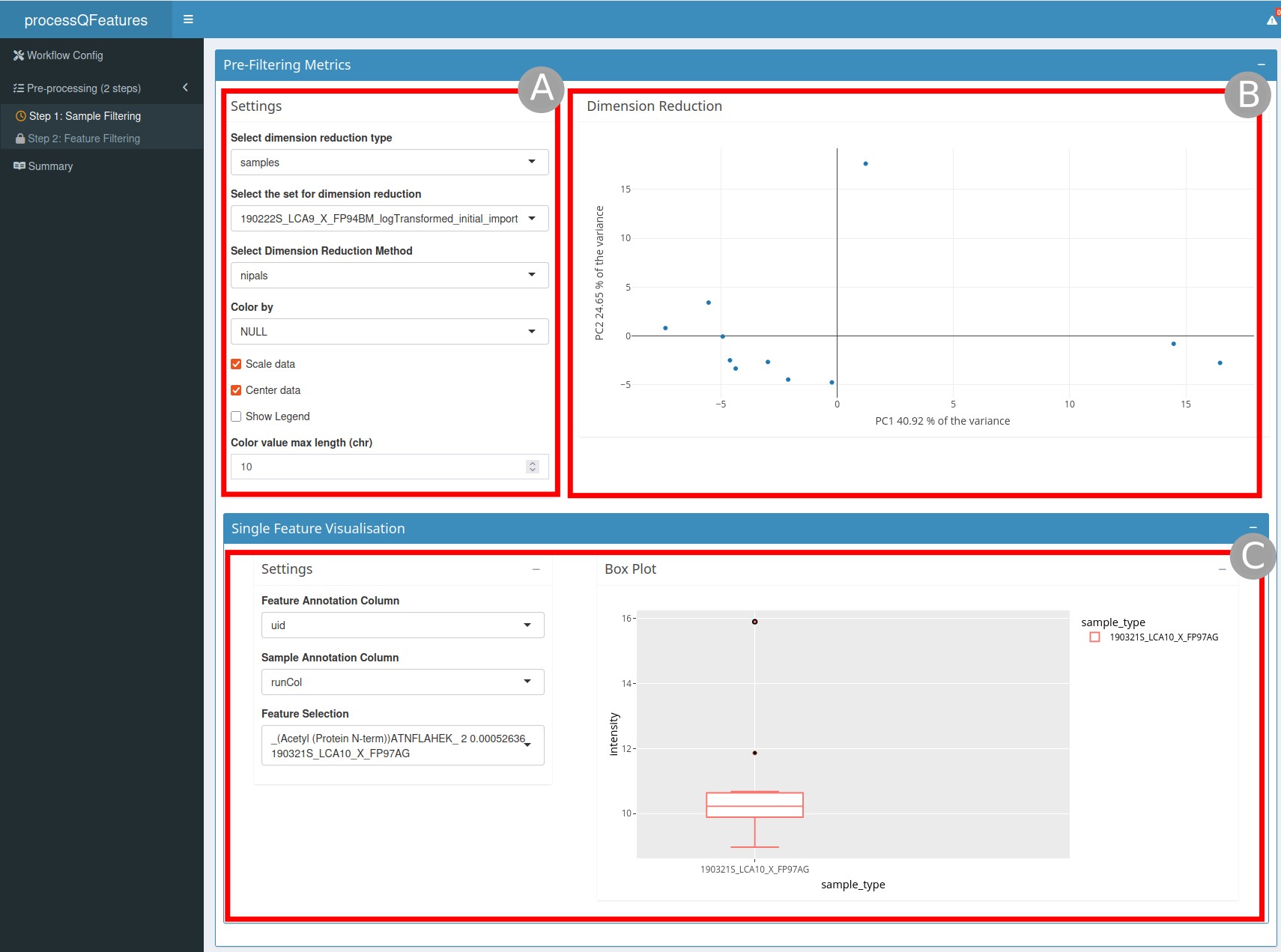
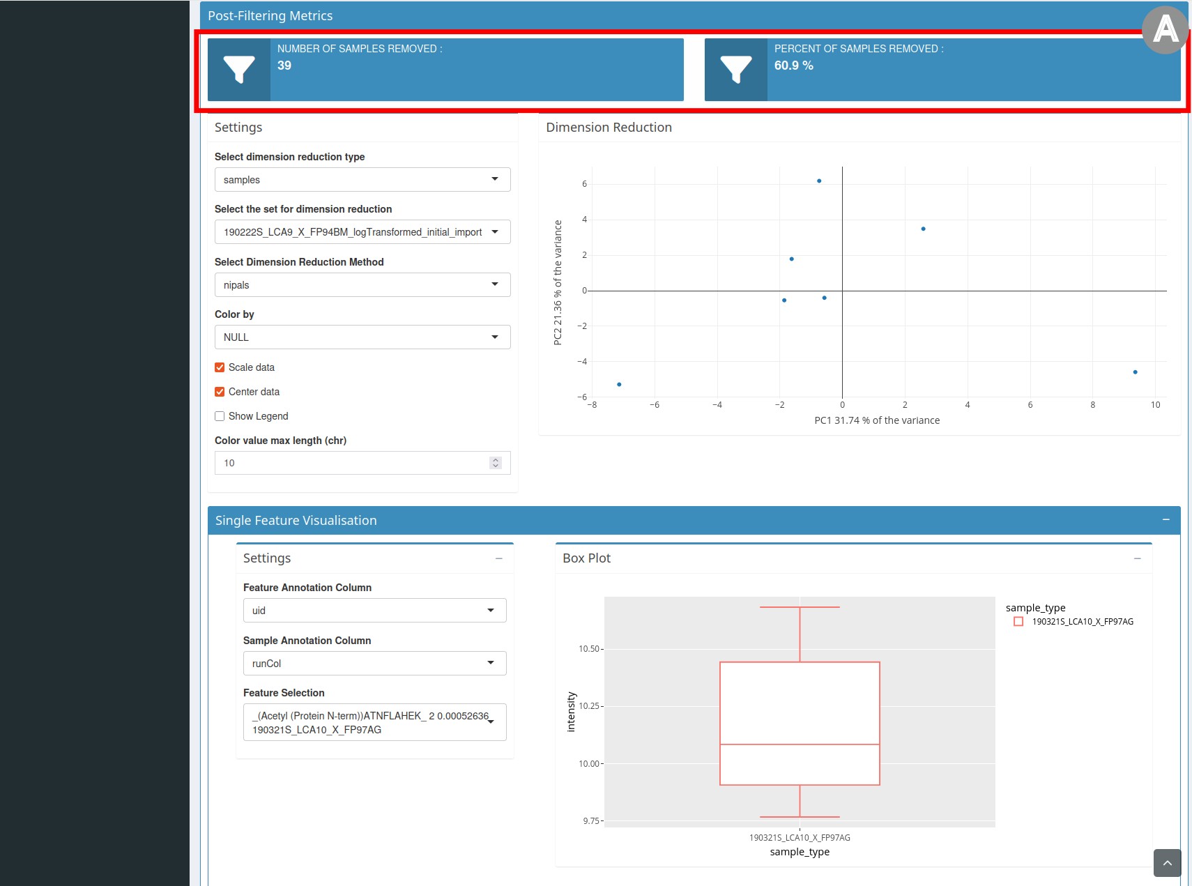
Pre-Filtering Metrics section

pre-Filtering metrics section

The Pre-Filtering Metrics section (Figure 1) is composed of two different parts:

• a dimension reduction graph (B) on the right and the settings (A) to customize this graph on the left. For example, you can choose the dimensionality reduction method or type.

• a single feature visualization (C) where you can display a boxplot of a selected feature split by sample annotation.

Filtering section

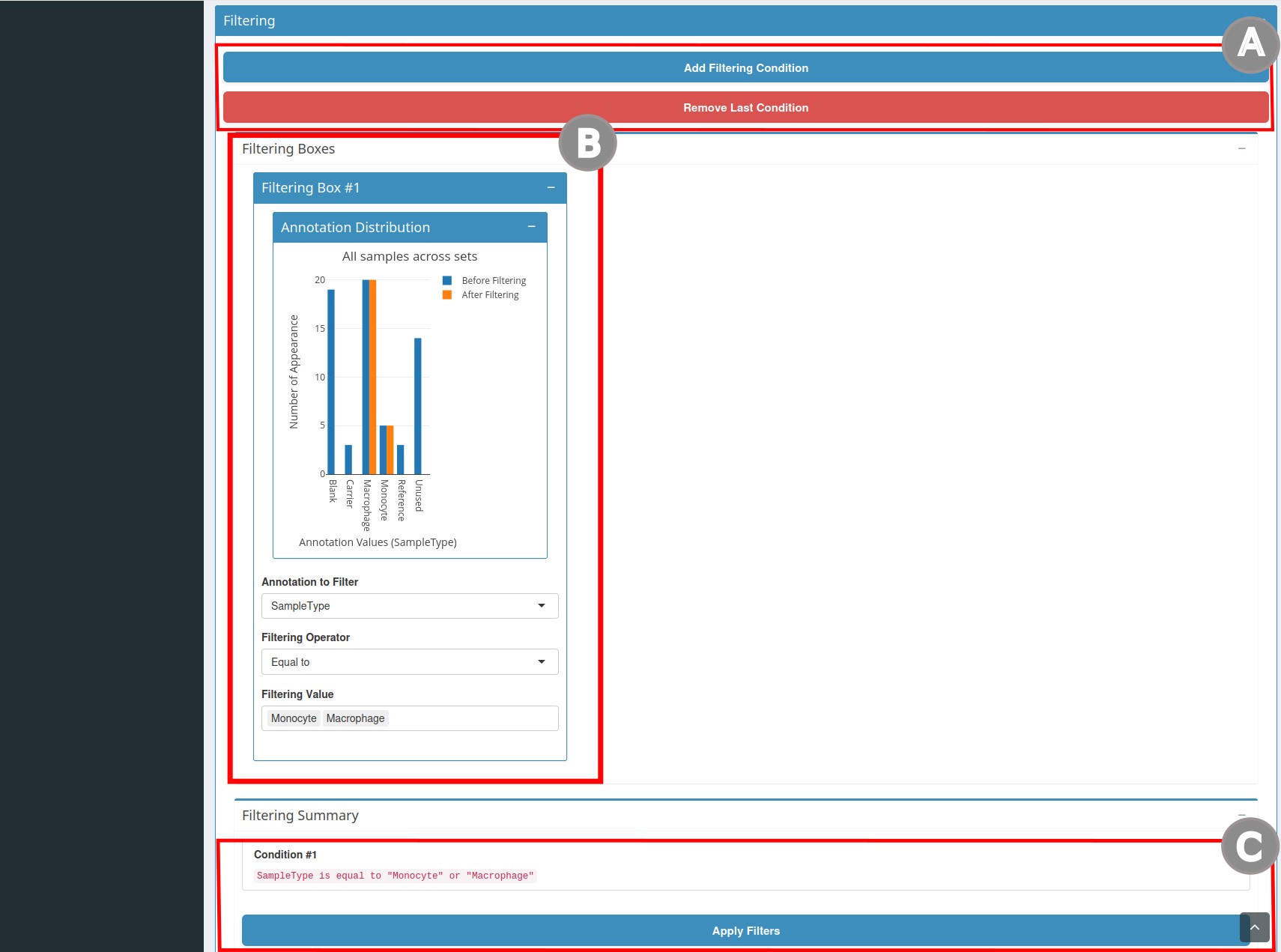
filtering section

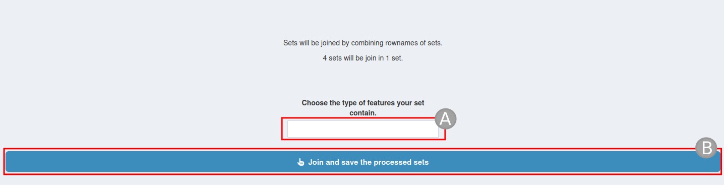
• The second section is Filtering (Figure 2). To create a condition, click Add Filtering Condition (A). Clicking this button will open the filtering boxes (B). In this box, you can add filtering conditions. Once you have chosen the annotation and the value to filter, the number of cells that will be filtered is updated dynamically. You will also find a summary of the selected conditions. Once the filters are chosen, click Apply Filters (C). If a condition is unnecessary, you can also click on Remove Last Condition (A).

Post-filtering Metrics section

post-Filtering metrics section

• The third section, entitled Post-Filtering Metrics (Figure 3), repeats the elements of the Pre-Filtering Metrics section, but the graph presents the data after filtering. It also contains statistics on the number and percentage of samples/features removed.

Once the filtering has been done, save the object by clicking the button Save the processed sets.

Filtering missing values by samples/features

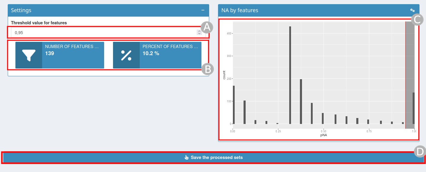
Filtering missing values by samples/features page

Missing values can be very numerous in certain proteomics experiments and need to be dealt with carefully.

In this step, you will need to define a threshold for the percentage of missing values (NA) beyond which a feature/sample should be removed (A). By changing this value, the statistics relating to the number and percentage of features/samples removed (B) and the associated graph (C) will be automatically updated. Once the threshold is defined, click on Save the processed sets (D).

Normalisation

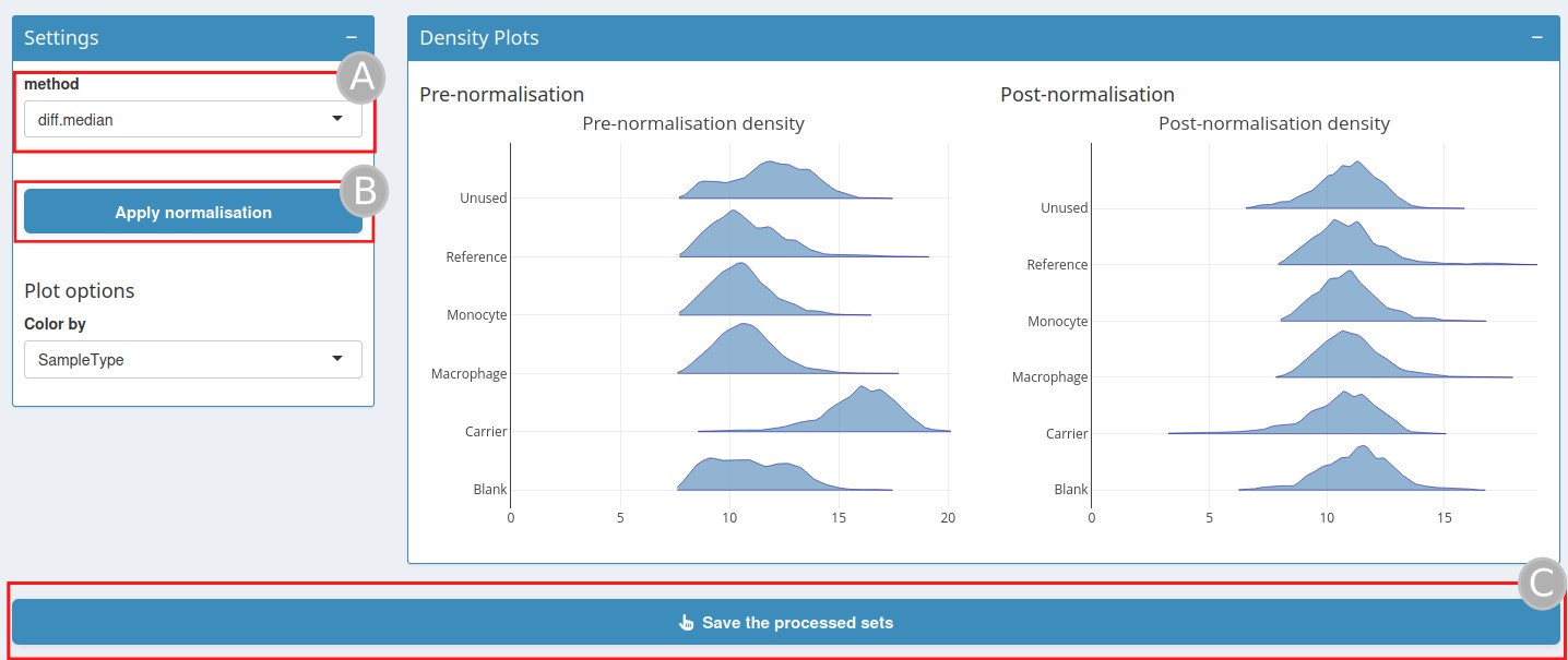
Normalization page

QFeatures objects can be normalised in this step. Several normalisation methods are available (A).

• sum and max, where each feature’s intensity is divided by the maximum or the sum of the feature, respectively. These two methods are applied along the features (rows).

• center.mean and center.median centre the respective sample (column) intensities by subtracting the respective column means or medians. div.mean and div.median divide by the column means or medians.

• diff.median centres all samples (columns) so that they all match the grand median by subtracting the respective column median differences from the grand median.

• Using quantiles or quantiles.robust applies (robust) quantile normalisation, as implemented in preprocessCore::normalize.quantiles() and preprocessCore::normalize.quantiles.robust(). vsn uses the vsn::vsn2() function. Note that the latter also glog-transforms the intensities. See the respective manuals for more details and function arguments.

Once the normalisation method is selected, click on Apply normalisation (B); the density graph after normalisation will be displayed. Click on Save the processed sets (C).

Zero to NA

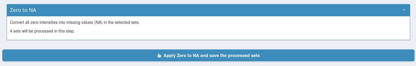
Zero to NA page

This step converts all zero intensities into missing values (NA) in the selected sets.

Log Transformation

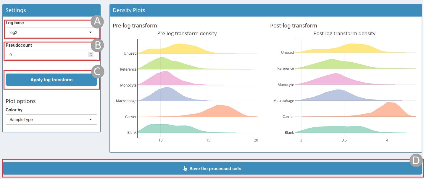
Log transformation page

When analysing continuous data using parametric methods (such as t-test or linear models), it is often necessary to log-transform the data.

The log base is set to log2 by default, but can also be set to log10 or ln (A). A pseudocount value can be added (B) to handle zero values in the data before applying the logarithm. Then click on Apply log transform (C); this will display a density plot after log transformation. Once this is done, do not forget to click on Save the processed sets (D).

Imputation

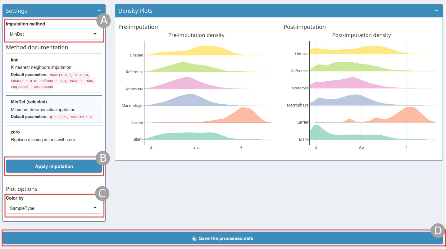
Imputation page

There are two types of mechanisms resulting in missing values in LC/MSMS experiments.

• Missing values resulting from the absence of detection of a feature, despite ions being present at detectable concentrations. For example, this can happen in the case of ion suppression or as a result of the stochastic, data-dependent nature of the MS acquisition method. These missing values are expected to be randomly distributed in the data and are defined as missing at random (MAR) or missing completely at random (MCAR).

• Biologically relevant missing values, resulting from the absence or low abundance of ions (below the limit of detection of the instrument). These missing values are not expected to be randomly distributed in the data and are defined as missing not at random (MNAR).

See Imputing quantitative proteomics data for more information.

First choose an imputation method (A):

• knn: nearest neighbour averaging, as implemented in the impute::impute.knn function. Note that this function is used with default parameters.

• MinDet: performs the imputation of left-censored missing data using a deterministic minimal value approach. Considering expression data with n samples and p features, for each sample, the missing entries are replaced with a minimal value observed in that sample. The minimal value observed is estimated as the q-th quantile (default q = 0.01) of the observed values in that sample. Implemented in imputeLCMD::impute.MinDet. Note that this function is used with default parameters.

• zero: replaces the missing values with 0.

Then click on Apply imputation (B). Once the imputation has run, the page will display a post-imputation density plot that you can colour by colData (C). Once the imputation step is finished, do not forget to Save the processed sets (D).

Aggregation

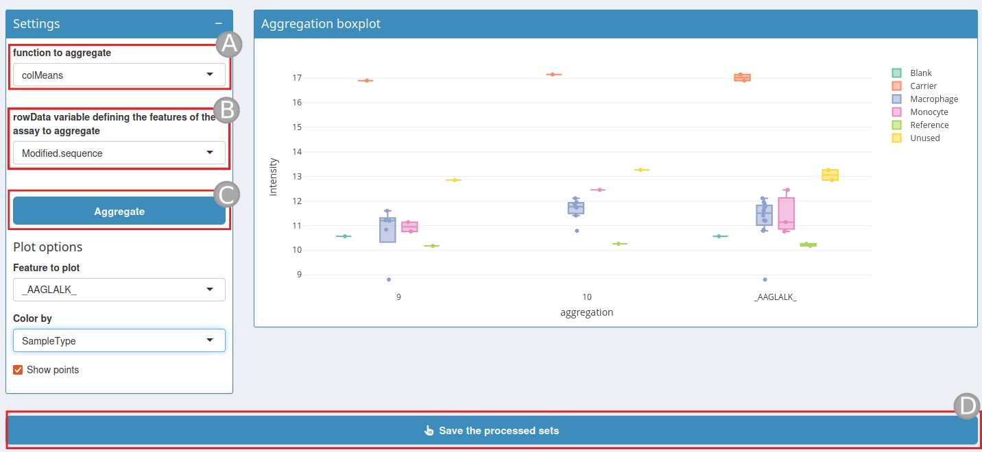
Aggregation page

At this stage, it is possible to use the peptide-level intensities or aggregate the peptide-level data into protein intensities.

To do this, a quantitative feature aggregation function is required. This function, called Function to aggregate (A), takes a matrix as input and returns a vector of length equal to ncol(x). The function can be one of the following types:

• MsCoreUtils::medianPolish() fits an additive model (two-way decomposition) using Tukey’s median polish procedure with stats::medpolish().

• MsCoreUtils::robustSummary calculates a robust aggregation using MASS::rlm() (default).

• base::colMeans() to use the mean of each column.

• matrixStats::colMedians() to use the median of each column.

• base::colSums() to use the sum of each column.

See MsCoreUtils::aggregate_by_vector() for more aggregation functions.

A rowData variable (B) is also needed to define how to aggregate the features of the assays.

Once these two variables have been set, click on Aggregate (C).

An aggregation boxplot will be displayed. This boxplot shows a feature coloured by a colData value. Once the aggregation is done, click on Save the processed sets.

Join

Join page

The Join tab will combine the results from the previous step into a single dataset for further analysis or export. Simply give it a new assay name (A). Then click Join and save the processed sets (B).

Summary

Summary page

The summary page displays the various assays present in the QFeatures object and indicates their interrelationships. Finally, a download button provides a zip file containing the final QFeatures object, the script used to generate it, and the R session with the package version.