Processing quantitative proteomics data with QFeatures

Abstract

This vignette describes how to process quantitative mass spectrometry data with QFeatures: cleaning up unneeded feature variables, adding an experimental design, filtering out contaminants and reverse hits, managing missing values, log-transforming, normalising and aggregating data. This vignette is distributed under a CC BY-SA license.

Reading data as `QFeatures`

We are going to use a subset of the CPTAC study 6 containing conditions A and B (Paulovich et al. 2010). The peptide-level data, as processed by MaxQuant (Cox and Mann 2008) is available in the msdata package:

basename(f <- msdata::quant(pattern = "cptac", full.names = TRUE))

## [1] "cptac_a_b_peptides.txt"

From the names of the columns, we see that the quantitative columns, starting with "Intensity." (note the dot!) are at positions 56 to 61.

x <- read.delim(f)
names(x)

##  [1] "Sequence"                 "N.term.cleavage.window"  
##  [3] "C.term.cleavage.window"   "Amino.acid.before"       
##  [5] "First.amino.acid"         "Second.amino.acid"       
##  [7] "Second.last.amino.acid"   "Last.amino.acid"         
##  [9] "Amino.acid.after"         "A.Count"                 
## [11] "R.Count"                  "N.Count"                 
## [13] "D.Count"                  "C.Count"                 
## [15] "Q.Count"                  "E.Count"                 
## [17] "G.Count"                  "H.Count"                 
## [19] "I.Count"                  "L.Count"                 
## [21] "K.Count"                  "M.Count"                 
## [23] "F.Count"                  "P.Count"                 
## [25] "S.Count"                  "T.Count"                 
## [27] "W.Count"                  "Y.Count"                 
## [29] "V.Count"                  "U.Count"                 
## [31] "Length"                   "Missed.cleavages"        
## [33] "Mass"                     "Proteins"                
## [35] "Leading.razor.protein"    "Start.position"          
## [37] "End.position"             "Unique..Groups."         
## [39] "Unique..Proteins."        "Charges"                 
## [41] "PEP"                      "Score"                   
## [43] "Identification.type.6A_7" "Identification.type.6A_8"
## [45] "Identification.type.6A_9" "Identification.type.6B_7"
## [47] "Identification.type.6B_8" "Identification.type.6B_9"
## [49] "Experiment.6A_7"          "Experiment.6A_8"         
## [51] "Experiment.6A_9"          "Experiment.6B_7"         
## [53] "Experiment.6B_8"          "Experiment.6B_9"         
## [55] "Intensity"                "Intensity.6A_7"          
## [57] "Intensity.6A_8"           "Intensity.6A_9"          
## [59] "Intensity.6B_7"           "Intensity.6B_8"          
## [61] "Intensity.6B_9"           "Reverse"                 
## [63] "Potential.contaminant"    "id"                      
## [65] "Protein.group.IDs"        "Mod..peptide.IDs"        
## [67] "Evidence.IDs"             "MS.MS.IDs"               
## [69] "Best.MS.MS"               "Oxidation..M..site.IDs"  
## [71] "MS.MS.Count"

(i <- grep("Intensity\\.", names(x)))

## [1] 56 57 58 59 60 61

We now read these data using the readQFeatures function. The peptide level expression data will be imported into R as an instance of class QFeatures named cptac with an assay named peptides. We also use the fnames argument to set the row-names of the peptides assay to the peptide sequences.

library("QFeatures")
cptac <- readQFeatures(x, quantCols = i, name = "peptides", fnames = "Sequence")

## Checking arguments.

## Loading data as a 'SummarizedExperiment' object.

## Formatting sample annotations (colData).

## Formatting data as a 'QFeatures' object.

## Setting assay rownames.

cptac

## An instance of class QFeatures containing 1 set(s):
##  [1] peptides: SummarizedExperiment with 11466 rows and 6 columns

Encoding the experimental design

Below we update the sample (column) annotations to encode the two groups, 6A and 6B, and the original sample numbers.

cptac$group <- rep(c("6A", "6B"), each = 3)
cptac$sample <- rep(7:9, 2)
colData(cptac)

## DataFrame with 6 rows and 2 columns
##                      group    sample
##                <character> <integer>
## Intensity.6A_7          6A         7
## Intensity.6A_8          6A         8
## Intensity.6A_9          6A         9
## Intensity.6B_7          6B         7
## Intensity.6B_8          6B         8
## Intensity.6B_9          6B         9

Filtering out contaminants and reverse hits

filterFeatures(cptac, ~ Reverse == "")

## 'Reverse' found in 1 out of 1 assay(s)

## An instance of class QFeatures containing 1 set(s):
##  [1] peptides: SummarizedExperiment with 11436 rows and 6 columns

filterFeatures(cptac, ~ Potential.contaminant == "")

## 'Potential.contaminant' found in 1 out of 1 assay(s)

## An instance of class QFeatures containing 1 set(s):
##  [1] peptides: SummarizedExperiment with 11385 rows and 6 columns

cptac <- cptac |>
    filterFeatures(~ Reverse == "") |>
    filterFeatures(~ Potential.contaminant == "")

## 'Reverse' found in 1 out of 1 assay(s)

## 'Potential.contaminant' found in 1 out of 1 assay(s)

Removing up unneeded feature variables

The spreadsheet that was read above contained numerous variables that are returned by MaxQuant, but not necessarily necessary in the frame of a downstream statistical analysis.

rowDataNames(cptac)

## CharacterList of length 1
## [["peptides"]] Sequence N.term.cleavage.window ... MS.MS.Count

The only ones that we will be needing below are the peptides sequences and the protein identifiers. Below, we store these variables of interest and filter them using the selectRowData function.

rowvars <- c("Sequence", "Proteins", "Leading.razor.protein")
cptac <- selectRowData(cptac, rowvars)
rowDataNames(cptac)

## CharacterList of length 1
## [["peptides"]] Sequence Proteins Leading.razor.protein

Managing missing values

Missing values can be very numerous in certain proteomics experiments and need to be dealt with carefully. The first step is to assess their presence across samples and features. But before being able to do so, we need to replace 0 by NA, given that MaxQuant encodes missing data with a 0 using the zeroIsNA function.

cptac <- zeroIsNA(cptac, i = seq_along(cptac))
nNA(cptac, i = seq_along(cptac))

## $nNA
## DataFrame with 1 row and 3 columns
##         assay       nNA       pNA
##   <character> <integer> <numeric>
## 1    peptides     30609  0.449194
## 
## $nNArows
## DataFrame with 11357 rows and 4 columns
##             assay          name       nNA       pNA
##       <character>   <character> <integer> <numeric>
## 1        peptides AAAAGAGGAG...         4  0.666667
## 2        peptides     AAAALAGGK         0  0.000000
## 3        peptides    AAAALAGGKK         0  0.000000
## 4        peptides AAADALSDLE...         0  0.000000
## 5        peptides AAADALSDLE...         0  0.000000
## ...           ...           ...       ...       ...
## 11353    peptides YYSIYDLGNN...         6  1.000000
## 11354    peptides YYTFNGPNYN...         3  0.500000
## 11355    peptides    YYTITEVATR         4  0.666667
## 11356    peptides YYTVFDRDNN...         6  1.000000
## 11357    peptides YYTVFDRDNN...         6  1.000000
## 
## $nNAcols
## DataFrame with 6 rows and 4 columns
##         assay          name       nNA       pNA
##   <character>   <character> <integer> <numeric>
## 1    peptides Intensity....      4669  0.411112
## 2    peptides Intensity....      5388  0.474421
## 3    peptides Intensity....      5224  0.459981
## 4    peptides Intensity....      4651  0.409527
## 5    peptides Intensity....      5470  0.481641
## 6    peptides Intensity....      5207  0.458484

The output of the nNA function tells us that

there are currently close to 50% is missing values in the data;
there are 4051 peptides with 0 missing values, 989 with a single missing values, … and 3014 peptides composed of only missing values;
the range of missing values in the 6 samples is comparable and ranges between 4651 and 5470.

In this dataset, we have such a high number of peptides without any data because the 6 samples are a subset of a larger dataset, and these peptides happened to be absent in groups A and B. Below, we use filterNA to remove all the peptides that contain one or more missing values by using pNA = 0 (which also is the default value).

cptac <- filterNA(cptac, i = seq_along(cptac), pNA = 0)
cptac

## An instance of class QFeatures containing 1 set(s):
##  [1] peptides: SummarizedExperiment with 4051 rows and 6 columns

I we wanted to keep peptides that have up to 90% of missing values, corresponsing in this case to those that have only one value (i.e 5/6 percent of missing values), we could have set pNA to 0.9.

Counting unique features

Counting the number of unique features across samples can be used for quality control or for assessing the identification efficiency between different conditions or experimental set-ups. countUniqueFeatures can be used to count the number of features that are contained in each sample of an assay from a QFeatures object. For instance, we can count the number of (non-missing) peptides per sample from the peptides assay. Note that the counts are automatically stored in the colData of cptac, under peptide_counts:

cptac <- countUniqueFeatures(cptac,
                             i = "peptides",
                             colDataName = "peptide_counts")
colData(cptac)

## DataFrame with 6 rows and 3 columns
##                      group    sample peptide_counts
##                <character> <integer>      <integer>
## Intensity.6A_7          6A         7           4051
## Intensity.6A_8          6A         8           4051
## Intensity.6A_9          6A         9           4051
## Intensity.6B_7          6B         7           4051
## Intensity.6B_8          6B         8           4051
## Intensity.6B_9          6B         9           4051

We can also count the number of unique proteins. We therefore need to tell countUniqueFeatures that we need to group by protein (the protein name is stored in the rowData under Proteins):

cptac <- countUniqueFeatures(cptac,
                             i = "peptides",
                             groupBy = "Proteins",
                             colDataName = "protein_counts")
colData(cptac)

## DataFrame with 6 rows and 4 columns
##                      group    sample peptide_counts protein_counts
##                <character> <integer>      <integer>      <integer>
## Intensity.6A_7          6A         7           4051           1125
## Intensity.6A_8          6A         8           4051           1125
## Intensity.6A_9          6A         9           4051           1125
## Intensity.6B_7          6B         7           4051           1125
## Intensity.6B_8          6B         8           4051           1125
## Intensity.6B_9          6B         9           4051           1125

Imputation

The impute method can be used to perform missing value imputation using a variety of imputation methods. The method takes an instance of class QFeatures (or a SummarizedExperiment) as input, an a character naming the desired method (see ?impute for the complete list with details) and returns a new instance of class QFeatures (or SummarizedExperiment) with imputed data.

As described in more details in (Lazar et al. 2016), there are two types of mechanisms resulting in missing values in LC/MSMS experiments.

Missing values resulting from absence of detection of a feature, despite ions being present at detectable concentrations. For example in the case of ion suppression or as a result from the stochastic, data-dependent nature of the MS acquisition method. These missing value are expected to be randomly distributed in the data and are defined as missing at random (MAR) or missing completely at random (MCAR).
Biologically relevant missing values, resulting from the absence of the low abundance of ions (below the limit of detection of the instrument). These missing values are not expected to be randomly distributed in the data and are defined as missing not at random (MNAR).

MAR and MCAR values can be reasonably well tackled by many imputation methods. MNAR data, however, requires some knowledge about the underlying mechanism that generates the missing data, to be able to attempt data imputation. MNAR features should ideally be imputed with a left-censor (for example using a deterministic or probabilistic minimum value) method. Conversely, it is recommended to use hot deck methods (for example nearest neighbour, maximum likelihood, etc) when data are missing at random.

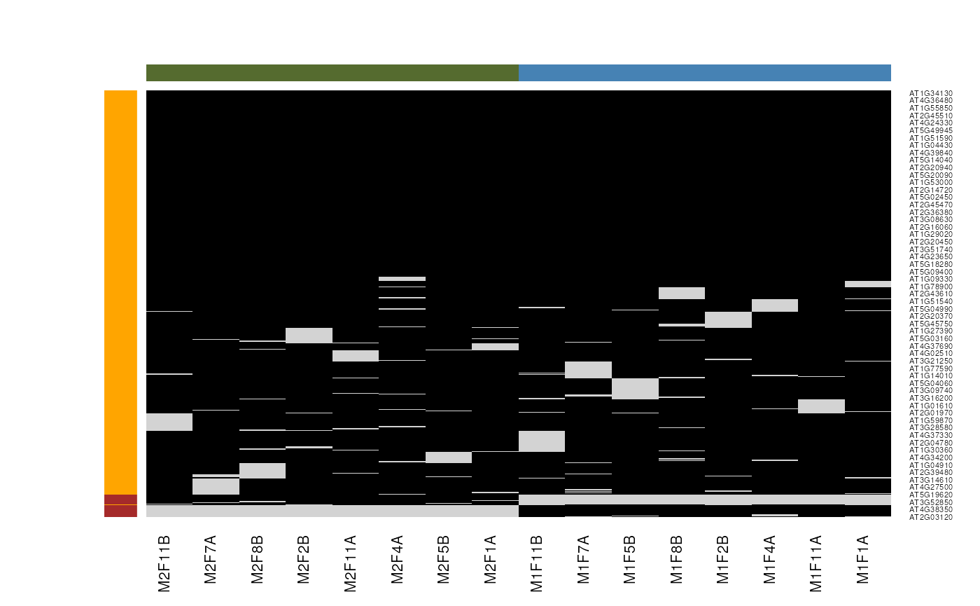
Mixed imputation method. Black cells represent presence of quantitation values and light grey corresponds to missing data. The two groups of interest are depicted in green and blue along the heatmap columns. Two classes of proteins are annotated on the left: yellow are proteins with randomly occurring missing values (if any) while proteins in brown are candidates for non-random missing value imputation.

It is anticipated that the identification of both classes of missing values will depend on various factors, such as feature intensities and experimental design. Below, we use perform mixed imputation, applying nearest neighbour imputation on the 654 features that are assumed to contain randomly distributed missing values (if any) (yellow on figure @ref(fig:miximp)) and a deterministic minimum value imputation on the 35 proteins that display a non-random pattern of missing values (brown on figure @ref(fig:miximp)).

Data transformation

When analysing continuous data using parametric methods (such as t-test or linear models), it is often necessary to log-transform the data. The figure below (left) show that how our data is mainly composed of small values with a long tail of larger ones, which is a typical pattern of quantitative omics data.

Below, we use the logTransform function to log2-transform our data. This time, instead of overwriting the peptides assay, we are going to create a new one to contain the log2-transformed data.

cptac <- addAssay(cptac,
                  logTransform(cptac[[1]]),
                  name = "peptides_log")
cptac

## An instance of class QFeatures containing 2 set(s):
##  [1] peptides: SummarizedExperiment with 4051 rows and 6 columns 
##  [2] peptides_log: SummarizedExperiment with 4051 rows and 6 columns

The addAssay() function is the general function that adds new assays to a QFeatures object. The step above could also be fun with the following syntax, that implicitly returns an updated QFeatures object.

logTransform(cptac,
             i = "peptides",
             name = "log_peptides")

par(mfrow = c(1, 2))
limma::plotDensities(assay(cptac[[1]]))
limma::plotDensities(assay(cptac[[2]]))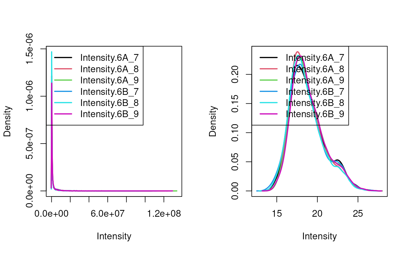

Quantitative data in its original scale (left) and log2-transformed (right).

Normalisation

Assays in QFeatures objects can be normalised with the normalize function. The type of normalisation is defined by the method argument; below, we use quantile normalisation, store the normalised data into a new experiment, and visualise the resulting data.

cptac <- addAssay(cptac,
                  normalize(cptac[["peptides_log"]], method = "center.median"),
                  name = "peptides_norm")
cptac

## An instance of class QFeatures containing 3 set(s):
##  [1] peptides: SummarizedExperiment with 4051 rows and 6 columns 
##  [2] peptides_log: SummarizedExperiment with 4051 rows and 6 columns 
##  [3] peptides_norm: SummarizedExperiment with 4051 rows and 6 columns

As above, the normalize() function can also be firectly applied to the QFeatures object.

normalize(cptac,
          i = "log_peptides",
          name = "lognorm_peptides",
          method = "center.median")

par(mfrow = c(1, 2))
limma::plotDensities(assay(cptac[["peptides_log"]]))
limma::plotDensities(assay(cptac[["peptides_norm"]]))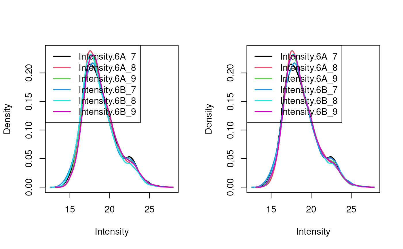

Distribution of log2 peptide intensities before (left) and after (right) median normalisation.

Feature aggregation

At this stage, it is possible to directly use the peptide-level intensities to perform a statistical analysis (Goeminne, Gevaert, and Clement 2016), or aggregate the peptide-level data into protein intensities, and perform the differential expression analysis at the protein level.

To aggregate feature data, we can use the aggregateFeatures function that takes the following inputs:

the name of the QFeatures instance that contains the peptide quantitation data - "cptac" in our example;
i: the name or index of the assay that contains the (normalised) peptide quantitation data - "peptides_norm" in our case;
fcol: the feature variable (in the assay above) to be used to define what peptides to aggregate - "Proteins" here, given that we want to aggregate all peptides that belong to one protein (group);
name: the name of the new aggregates assay - "proteins" in this case;
and finally fun, the function that will compute this aggregation - we will be using the default value, namely robustSummary (Sticker et al. 2019).

cptac <- aggregateFeatures(cptac, i = "peptides_norm", fcol = "Proteins", name = "proteins")
cptac

## An instance of class QFeatures containing 4 set(s):
##  [1] peptides: SummarizedExperiment with 4051 rows and 6 columns 
##  [2] peptides_log: SummarizedExperiment with 4051 rows and 6 columns 
##  [3] peptides_norm: SummarizedExperiment with 4051 rows and 6 columns 
##  [4] proteins: SummarizedExperiment with 1125 rows and 6 columns

We obtain a final 1125 quantified proteins in the new proteins assay. Below, we display the quantitation data for the first 6 proteins and their respective variables. The latter shown that number of peptides that were using during the aggregation step (.n column).

head(assay(cptac[["proteins"]]))

##                                      Intensity.6A_7 Intensity.6A_8
## P00918ups|CAH2_HUMAN_UPS                 -1.1215216      -1.379182
## P01008ups|ANT3_HUMAN_UPS;CON__P41361     -1.5422314      -2.248132
## P01127ups|PDGFB_HUMAN_UPS                -1.9097789      -1.459409
## P02144ups|MYG_HUMAN_UPS                  -1.5447867      -1.802439
## P02753ups|RETBP_HUMAN_UPS                -0.5570714      -1.565853
## P02787ups|TRFE_HUMAN_UPS                 -1.6165226      -1.387464
##                                      Intensity.6A_9 Intensity.6B_7
## P00918ups|CAH2_HUMAN_UPS                  -1.729731    -0.08402797
## P01008ups|ANT3_HUMAN_UPS;CON__P41361      -2.027588    -1.64110874
## P01127ups|PDGFB_HUMAN_UPS                 -1.526767    -0.16310747
## P02144ups|MYG_HUMAN_UPS                   -1.081029    -0.49570667
## P02753ups|RETBP_HUMAN_UPS                 -1.806130     0.03241792
## P02787ups|TRFE_HUMAN_UPS                  -2.014992    -0.22328799
##                                      Intensity.6B_8 Intensity.6B_9
## P00918ups|CAH2_HUMAN_UPS                  0.1874563     0.10613700
## P01008ups|ANT3_HUMAN_UPS;CON__P41361     -1.6201035    -1.88043072
## P01127ups|PDGFB_HUMAN_UPS                 0.4099189    -1.19416255
## P02144ups|MYG_HUMAN_UPS                   0.1929367    -0.06935162
## P02753ups|RETBP_HUMAN_UPS                -0.6263334    -0.20902837
## P02787ups|TRFE_HUMAN_UPS                  0.1491834    -0.20422237

rowData(cptac[["proteins"]])

## DataFrame with 1125 rows and 3 columns
##                                           Proteins Leading.razor.protein
##                                        <character>           <character>
## P00918ups|CAH2_HUMAN_UPS             P00918ups|...         P00918ups|...
## P01008ups|ANT3_HUMAN_UPS;CON__P41361 P01008ups|...         P01008ups|...
## P01127ups|PDGFB_HUMAN_UPS            P01127ups|...         P01127ups|...
## P02144ups|MYG_HUMAN_UPS              P02144ups|...         P02144ups|...
## P02753ups|RETBP_HUMAN_UPS            P02753ups|...         P02753ups|...
## ...                                            ...                   ...
## sp|Q99207|NOP14_YEAST                sp|Q99207|...         sp|Q99207|...
## sp|Q99216|PNO1_YEAST                 sp|Q99216|...         sp|Q99216|...
## sp|Q99257|MEX67_YEAST                sp|Q99257|...         sp|Q99257|...
## sp|Q99258|RIB3_YEAST                 sp|Q99258|...         sp|Q99258|...
## sp|Q99383|HRP1_YEAST                 sp|Q99383|...         sp|Q99383|...
##                                             .n
##                                      <integer>
## P00918ups|CAH2_HUMAN_UPS                     1
## P01008ups|ANT3_HUMAN_UPS;CON__P41361         1
## P01127ups|PDGFB_HUMAN_UPS                    1
## P02144ups|MYG_HUMAN_UPS                      1
## P02753ups|RETBP_HUMAN_UPS                    2
## ...                                        ...
## sp|Q99207|NOP14_YEAST                        1
## sp|Q99216|PNO1_YEAST                         1
## sp|Q99257|MEX67_YEAST                        2
## sp|Q99258|RIB3_YEAST                         2
## sp|Q99383|HRP1_YEAST                         2

We can get a quick overview of this .n variable by computing the table below, that shows us that we have 405 proteins that are based on a single peptides, 230 that are based on two, 119 that are based on three, … and a single protein that is the results of aggregating 44 peptides.

table(rowData(cptac[["proteins"]])$.n)

## 
##   1   2   3   4   5   6   7   8   9  10  11  12  13  14  15  16  17  18  19  20 
## 405 230 119  84  64  53  37  29  24  24  13   9   4   3   3   7   3   1   1   1 
##  21  22  23  24  25  30  31  33  44 
##   1   2   2   1   1   1   1   1   1

Let’s choose P02787ups|TRFE_HUMAN_UPS and visualise its expression pattern in the 2 groups at the protein and peptide level.

library("ggplot2")
library("dplyr")
longFormat(cptac["P02787ups|TRFE_HUMAN_UPS", ]) |>
    as.data.frame() |>
    mutate(group = ifelse(grepl("A", colname), "A", "B")) |>
    mutate(sample = sub("Intensity\\.", "", colname)) |>
    ggplot(aes(x = sample, y = value, colour = rowname, shape = group)) +
    geom_point() +
    facet_grid(~ assay)

## harmonizing input:
##   removing 12 sampleMap rows not in names(experiments)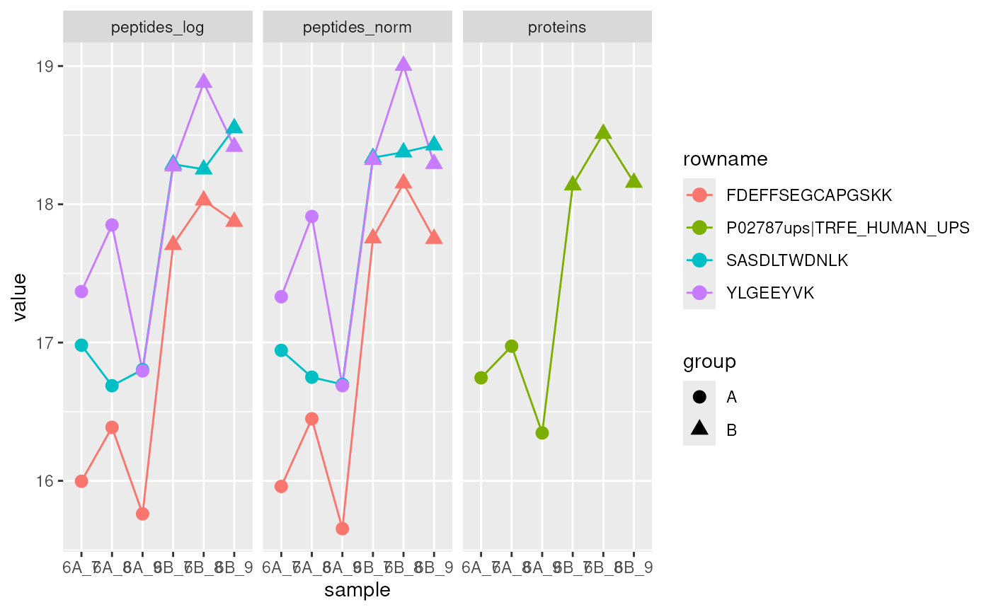

## Warning in lifeCycle("longForm", package = "MultiAssayExperiment", title = "longFormat"): 'longFormat' is deprecated.
##   Use 'longForm' instead.
##   See help('longFormat-deprecated').

Expression intensities for the protein P02787ups|TRFE_HUMAN_UPS (right, green) and its peptides (left) in groups A (circles) and B (triangles).

TODO

Improve on data visualisation.

Session information

## R Under development (unstable) (2025-02-24 r87814)
## Platform: x86_64-pc-linux-gnu
## Running under: Ubuntu 24.04.2 LTS
## 
## Matrix products: default
## BLAS:   /usr/lib/x86_64-linux-gnu/openblas-pthread/libblas.so.3 
## LAPACK: /usr/lib/x86_64-linux-gnu/openblas-pthread/libopenblasp-r0.3.26.so;  LAPACK version 3.12.0
## 
## locale:
##  [1] LC_CTYPE=en_US.UTF-8       LC_NUMERIC=C              
##  [3] LC_TIME=en_US.UTF-8        LC_COLLATE=en_US.UTF-8    
##  [5] LC_MONETARY=en_US.UTF-8    LC_MESSAGES=en_US.UTF-8   
##  [7] LC_PAPER=en_US.UTF-8       LC_NAME=C                 
##  [9] LC_ADDRESS=C               LC_TELEPHONE=C            
## [11] LC_MEASUREMENT=en_US.UTF-8 LC_IDENTIFICATION=C       
## 
## time zone: UTC
## tzcode source: system (glibc)
## 
## attached base packages:
## [1] stats4    stats     graphics  grDevices utils     datasets  methods  
## [8] base     
## 
## other attached packages:
##  [1] gplots_3.2.0                dplyr_1.1.4                
##  [3] ggplot2_3.5.1               QFeatures_1.17.5           
##  [5] MultiAssayExperiment_1.33.9 SummarizedExperiment_1.37.0
##  [7] Biobase_2.67.0              GenomicRanges_1.59.1       
##  [9] GenomeInfoDb_1.43.4         IRanges_2.41.3             
## [11] S4Vectors_0.45.4            BiocGenerics_0.53.6        
## [13] generics_0.1.3              MatrixGenerics_1.19.1      
## [15] matrixStats_1.5.0           BiocStyle_2.35.0           
## 
## loaded via a namespace (and not attached):
##  [1] tidyselect_1.2.1        farver_2.1.2            bitops_1.0-9           
##  [4] fastmap_1.2.0           lazyeval_0.2.2          digest_0.6.37          
##  [7] lifecycle_1.0.4         cluster_2.1.8           ProtGenerics_1.39.2    
## [10] statmod_1.5.0           magrittr_2.0.3          compiler_4.5.0         
## [13] rlang_1.1.5             sass_0.4.9              tools_4.5.0            
## [16] igraph_2.1.4            yaml_2.3.10             knitr_1.50             
## [19] labeling_0.4.3          S4Arrays_1.7.3          htmlwidgets_1.6.4      
## [22] DelayedArray_0.33.6     plyr_1.8.9              abind_1.4-8            
## [25] KernSmooth_2.23-26      withr_3.0.2             purrr_1.0.4            
## [28] desc_1.4.3              grid_4.5.0              caTools_1.18.3         
## [31] colorspace_2.1-1        scales_1.3.0            gtools_3.9.5           
## [34] MASS_7.3-65             cli_3.6.4               rmarkdown_2.29         
## [37] crayon_1.5.3            ragg_1.3.3              httr_1.4.7             
## [40] reshape2_1.4.4          BiocBaseUtils_1.9.0     cachem_1.1.0           
## [43] stringr_1.5.1           AnnotationFilter_1.31.0 BiocManager_1.30.25    
## [46] XVector_0.47.2          vctrs_0.6.5             Matrix_1.7-2           
## [49] jsonlite_1.9.1          bookdown_0.42           clue_0.3-66            
## [52] systemfonts_1.2.1       limma_3.63.10           tidyr_1.3.1            
## [55] jquerylib_0.1.4         glue_1.8.0              pkgdown_2.1.1.9000     
## [58] stringi_1.8.4           gtable_0.3.6            UCSC.utils_1.3.1       
## [61] munsell_0.5.1           tibble_3.2.1            pillar_1.10.1          
## [64] htmltools_0.5.8.1       GenomeInfoDbData_1.2.14 R6_2.6.1               
## [67] textshaping_1.0.0       evaluate_1.0.3          lattice_0.22-6         
## [70] msdata_0.47.0           bslib_0.9.0             Rcpp_1.0.14            
## [73] SparseArray_1.7.7       xfun_0.51               MsCoreUtils_1.19.1     
## [76] fs_1.6.5                pkgconfig_2.0.3

References

Cox, J, and M Mann. 2008. “MaxQuant Enables High Peptide Identification Rates, Individualized p.p.b.-Range Mass Accuracies and Proteome-Wide Protein Quantification.” Nat Biotechnol 26 (12): 1367–72. https://doi.org/10.1038/nbt.1511.

Goeminne, L J, K Gevaert, and L Clement. 2016. “Peptide-Level Robust Ridge Regression Improves Estimation, Sensitivity, and Specificity in Data-Dependent Quantitative Label-Free Shotgun Proteomics.” Mol Cell Proteomics 15 (2): 657–68. https://doi.org/10.1074/mcp.M115.055897.

Lazar, C, L Gatto, M Ferro, C Bruley, and T Burger. 2016. “Accounting for the Multiple Natures of Missing Values in Label-Free Quantitative Proteomics Data Sets to Compare Imputation Strategies.” J Proteome Res 15 (4): 1116–25. https://doi.org/10.1021/acs.jproteome.5b00981.

Paulovich, Amanda G, Dean Billheimer, Amy-Joan L Ham, Lorenzo Vega-Montoto, Paul A Rudnick, David L Tabb, Pei Wang, et al. 2010. “Interlaboratory Study Characterizing a Yeast Performance Standard for Benchmarking LC-MS Platform Performance.” Mol. Cell. Proteomics 9 (2): 242–54.

Sticker, Adriaan, Ludger Goeminne, Lennart Martens, and Lieven Clement. 2019. “Robust Summarization and Inference in Proteome-Wide Label-Free Quantification.” bioRxiv. https://doi.org/10.1101/668863.

Laurent Gatto

Reading data as `QFeatures`

Encoding the experimental design

Filtering out contaminants and reverse hits

Removing up unneeded feature variables

Managing missing values

Counting unique features

Imputation

Data transformation

Normalisation

Feature aggregation

TODO

See also

Session information

References

Processing quantitative proteomics data with QFeatures

Laurent Gatto

Reading data as QFeatures

Encoding the experimental design

Filtering out contaminants and reverse hits

Removing up unneeded feature variables

Managing missing values

Counting unique features

Imputation

Data transformation

Normalisation

Feature aggregation

TODO

See also

Session information

References

Reading data as `QFeatures`