Load mass spectrometry-based proteomics data using `readQFeatures()`

The `QFeatures` class

The QFeatures class stores data as a list of SummarizedExperiment objects that contain data processed at different levels. For instance, a QFeatures object may contain data at the peptide-to-spectrum-match (PSM) level, at the peptide level and at the protein level. We call each SummarizedExperiment object contained in a QFeatures object a set. Because the different sets are often related, they often share the same samples (columns). QFeatures automatically creates links between the related samples and their annotations (stored in a single colData table). Similarly, different sets often share related features (rows). For instance, proteins are composed of peptides and peptides are composed of PSMs. QFeatures automatically creates links between the related features through an AssayLinks object.

The `QFeatures` data class. The `QFeatures` object contains a list of `SummarizedExperiment` ojects (see [class description](https://bioconductor.org/packages/release/bioc/vignettes/SummarizedExperiment/inst/doc/SummarizedExperiment.html)) on `SingleCellExperiment` and `QFeatures` objects

The QFeatures data class. The QFeatures object contains a list of SummarizedExperiment ojects (see class description) on SingleCellExperiment and QFeatures objects

library("QFeatures")

Converting tabular data

QFeatures is designed to process and manipulate the MS-based proteomics data obtained after identification and quantification of the raw MS files. The identification and quantification steps are generally performed by dedicated software (e.g. Sage, FragPipe, Proteome Discoverer, MaxQuant, …) that return a set of tabular data. readQFeatures() converts these tabular data into a QFeatures object. We refer to these tables as the assayData tables.

We distinguish between two use cases: the single-set case and the multi-set case.

The single-set case

The single-set case will generate a QFeatures object with a single SummarizedExperiment object. This is generally the case when reading data at the peptide or protein level, or when the samples where multiplexed (e.g. using TMT) within a single MS run. There are two types of columns:

Quantitative columns (quantCols): 1 to n (depending on technology)
Feature annotations: e.g. peptide sequence, ion charge, protein name

In this case, each quantitative column contains information for a single sample. This can be schematically represented as below:

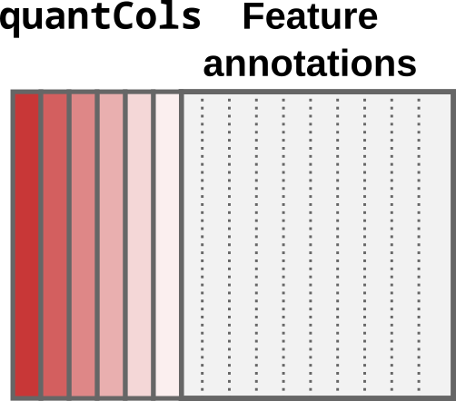
Schematic representation of a data table under the single-set case. Quantification columns (quantCols) are represented by different shades of red.

The hyperLOPIT data is an example data that falls under the single-set case (see ?hlpsms for more details). The quantCols are X126, X127N, X127C, …, X130N, X130C, X131 and correspond to different TMT labels.

In this toy example, there are 3,010 rows corresponding to features (quantified PSMs) and 28 columns corresponding to different data fields generated by MaxQuant during the analysis of the raw MS spectra. The table is converted to a QFeatures object as follows:

data("hlpsms")
quantCols <- grep("^X", colnames(hlpsms))
(qfSingle <- readQFeatures(hlpsms, quantCols = quantCols))
#> Checking arguments.
#> Loading data as a 'SummarizedExperiment' object.
#> Formatting sample annotations (colData).
#> Formatting data as a 'QFeatures' object.
#> An instance of class QFeatures containing 1 set(s):
#>  [1] quants: SummarizedExperiment with 3010 rows and 10 columns

The object returned by readQFeatures() is a QFeatures object containing 1 SummarizedExperiment set. The set is named quants by default, but we could name it psms by providing the name argument:

(qfSingle <- readQFeatures(hlpsms, quantCols = quantCols, name = "psms"))
#> Checking arguments.
#> Loading data as a 'SummarizedExperiment' object.
#> Formatting sample annotations (colData).
#> Formatting data as a 'QFeatures' object.
#> An instance of class QFeatures containing 1 set(s):
#>  [1] psms: SummarizedExperiment with 3010 rows and 10 columns

The multi-set case

The multi-set case will generate a QFeatures object with multiple SummarizedExperiment objects. This is generally the case when reading data at the PSM level that has been acquired as part of multiple runs. In this case, the identification and quantification software concatenates the results across MS runs in a single table. There are three types of columns:

Run identifier column (runCol): e.g. file name.
Quantification columns (quantCols): 1 to n (depending on technology).
Feature annotations: e.g. peptide sequence, ion charge, protein name.

Each quantitative column contains information for multiple samples. This can be schematically represented as below:

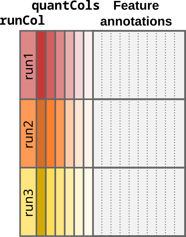
Schematic representation of a data table under the multi-set case. Quantification columns (quantCols) are coloured by run and shaded by label. Every sample is uniquely represented by a colour and shade. Note that every quantCol contains multiple samples.

We will again use hyperLOPIT data and simulate it was acquired as part of multiple runs, hence falling under the multi-set case. The MS run is often identified with the name of the file it generated.

hlpsms$FileName <- rep(
    rep(paste0("run", 1:3, ".raw"), each = 4), 
    length.out = nrow(hlpsms)
)

Note that the data set now has a column called “FileName” with 3 different runs:

To avoid that a quantification column contains data from multiple samples, readQFeatures() splits the table into mulitple set depending on the runCol column, here given as FileName:

(qfMulti <- readQFeatures(hlpsms, quantCols = quantCols, runCol = "FileName"))
#> Checking arguments.
#> Loading data as a 'SummarizedExperiment' object.
#> Splitting data in runs.
#> Formatting sample annotations (colData).
#> Formatting data as a 'QFeatures' object.
#> An instance of class QFeatures containing 3 set(s):
#>  [1] run1.raw: SummarizedExperiment with 1004 rows and 10 columns 
#>  [2] run2.raw: SummarizedExperiment with 1004 rows and 10 columns 
#>  [3] run3.raw: SummarizedExperiment with 1002 rows and 10 columns

The object returned by readQFeatures() is a QFeatures object containing 3 SummarizedExperiment sets. The sets are automatically named based on the values found in runCol.

Including sample annotations

Data often comes with sample annotations that provide information about the experimental design. These data are generally created by the user. To facilitate sample annotations, readQFeatures() also allows providing the annotation table as the colData argument. Depending on the use case, one or multiple columns are required.

For the single-set case, the colData table must contain a column named quantCols.

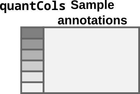
colData for the single-set case

Let’s simulate such a table:

(coldata <- DataFrame(
    quantCols = quantCols, 
    condition = rep(c("A", "B"), 5), 
    batch = rep(c("batch1", "batch2"), each = 5)
))
#> DataFrame with 10 rows and 3 columns
#>    quantCols   condition       batch
#>    <integer> <character> <character>
#> 1          1           A      batch1
#> 2          2           B      batch1
#> 3          3           A      batch1
#> 4          4           B      batch1
#> 5          5           A      batch1
#> 6          6           B      batch2
#> 7          7           A      batch2
#> 8          8           B      batch2
#> 9          9           A      batch2
#> 10        10           B      batch2

We can now provide the table to readQFeatures():

(qfSingle <- readQFeatures(hlpsms, quantCols = quantCols, colData = coldata))
#> Checking arguments.
#> Loading data as a 'SummarizedExperiment' object.
#> Formatting sample annotations (colData).
#> Formatting data as a 'QFeatures' object.
#> An instance of class QFeatures containing 1 set(s):
#>  [1] quants: SummarizedExperiment with 3010 rows and 10 columns

For convenience, the quantCols argument can be omitted when providing colData (quantCols are then fetched from this table):

(qfSingle <- readQFeatures(hlpsms, colData = coldata))
#> Checking arguments.
#> Loading data as a 'SummarizedExperiment' object.
#> Formatting sample annotations (colData).
#> Formatting data as a 'QFeatures' object.
#> An instance of class QFeatures containing 1 set(s):
#>  [1] quants: SummarizedExperiment with 3010 rows and 10 columns

The annotations are retrieved as follows:

colData(qfSingle)
#> DataFrame with 10 rows and 3 columns
#>       quantCols   condition       batch
#>       <integer> <character> <character>
#> X126          1           A      batch1
#> X127C         2           B      batch1
#> X127N         3           A      batch1
#> X128C         4           B      batch1
#> X128N         5           A      batch1
#> X129C         6           B      batch2
#> X129N         7           A      batch2
#> X130C         8           B      batch2
#> X130N         9           A      batch2
#> X131         10           B      batch2

For the multi-set case, the colData table must contain a column named quantCols and a column called runCol.

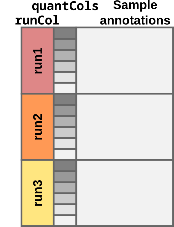
colData for the multi-set case

Let’s simulate an annotation table based on our previous example by duplicating the table for each run:

coldataMulti <- DataFrame()
for (run in paste0("run", 1:3, ".raw")) {
    coldataMulti <- rbind(coldataMulti, DataFrame(runCol = run, coldata))
}
coldataMulti
#> DataFrame with 30 rows and 4 columns
#>          runCol quantCols   condition       batch
#>     <character> <integer> <character> <character>
#> 1      run1.raw         1           A      batch1
#> 2      run1.raw         2           B      batch1
#> 3      run1.raw         3           A      batch1
#> 4      run1.raw         4           B      batch1
#> 5      run1.raw         5           A      batch1
#> ...         ...       ...         ...         ...
#> 26     run3.raw         6           B      batch2
#> 27     run3.raw         7           A      batch2
#> 28     run3.raw         8           B      batch2
#> 29     run3.raw         9           A      batch2
#> 30     run3.raw        10           B      batch2

We can provide the table to readQFeatures():

(qfMulti <- readQFeatures(
    hlpsms, quantCols = quantCols, colData = coldataMulti, 
    runCol = "FileName"
))
#> Checking arguments.
#> Loading data as a 'SummarizedExperiment' object.
#> Splitting data in runs.
#> Formatting sample annotations (colData).
#> Formatting data as a 'QFeatures' object.
#> An instance of class QFeatures containing 3 set(s):
#>  [1] run1.raw: SummarizedExperiment with 1004 rows and 10 columns 
#>  [2] run2.raw: SummarizedExperiment with 1004 rows and 10 columns 
#>  [3] run3.raw: SummarizedExperiment with 1002 rows and 10 columns

Additional information

Sample names

readQFeatures() automatically assigns names that are unique across all samples in all sets. In the single-set case, sample names are provided by quantCols.

colnames(qfSingle)
#> CharacterList of length 1
#> [["quants"]] X126 X127C X127N X128C X128N X129C X129N X130C X130N X131

In the multi-set case, sample names are the concatenation of the run name and the quantCols (separated by a _).

colnames(qfMulti)
#> CharacterList of length 3
#> [["run1.raw"]] run1.raw_X126 run1.raw_X127C ... run1.raw_X130N run1.raw_X131
#> [["run2.raw"]] run2.raw_X126 run2.raw_X127C ... run2.raw_X130N run2.raw_X131
#> [["run3.raw"]] run3.raw_X126 run3.raw_X127C ... run3.raw_X130N run3.raw_X131

Special case: empty samples

In some rare cases, it can be beneficial to remove samples where all quantifications are NA. This can occur when the raw data are searched for labels that were not used during the experiment. For instance, some may quantifying the raw data expecting TMT-16 labelling while the experiment used TMT-11 labels, or used half of the TMT-16 labels. The missing label channels are filled with NAs. When setting removeEmptyCols = TRUE, readQFeatures() automatically detects and removes columns containing only NAs.

hlpsms$X126 <- NA
(qfNoEmptyCol <- readQFeatures(
    hlpsms, quantCols = quantCols, removeEmptyCols = TRUE
))
#> Checking arguments.
#> Loading data as a 'SummarizedExperiment' object.
#> Formatting sample annotations (colData).
#> Formatting data as a 'QFeatures' object.
#> An instance of class QFeatures containing 1 set(s):
#>  [1] quants: SummarizedExperiment with 3010 rows and 9 columns

Note that we have set all values in X126 to missing. Hence, the set contains only 9 columns instead of the previous 10.

Reducing verbose

Every call to readQFeatures() prints progression to the console. To disable the console output, you can use the verbose argument:

(qfSingle <- readQFeatures(
    hlpsms, quantCols = quantCols, verbose = FALSE
))
#> An instance of class QFeatures containing 1 set(s):
#>  [1] quants: SummarizedExperiment with 3010 rows and 10 columns

Under the hood

readQFeatures proceeds as follows:

The assayData table must be provided as a data.frame (or any format that can be coerced to a data.frame). readQFeatures() converts the table to a SingleCellExperiment object using quantCols to identify the quantitative values that are stored in the assay slot. Any other column is considered as feature annotation and will be stored as rowData.

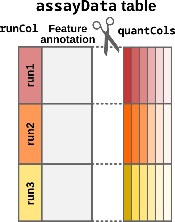
Step1: Convert the input table to a SingleCellExperiment object

(Only for the multi-set case:) The SingleCellExperiment object is split according to the acquisition run provided by the runCol column in assayData.

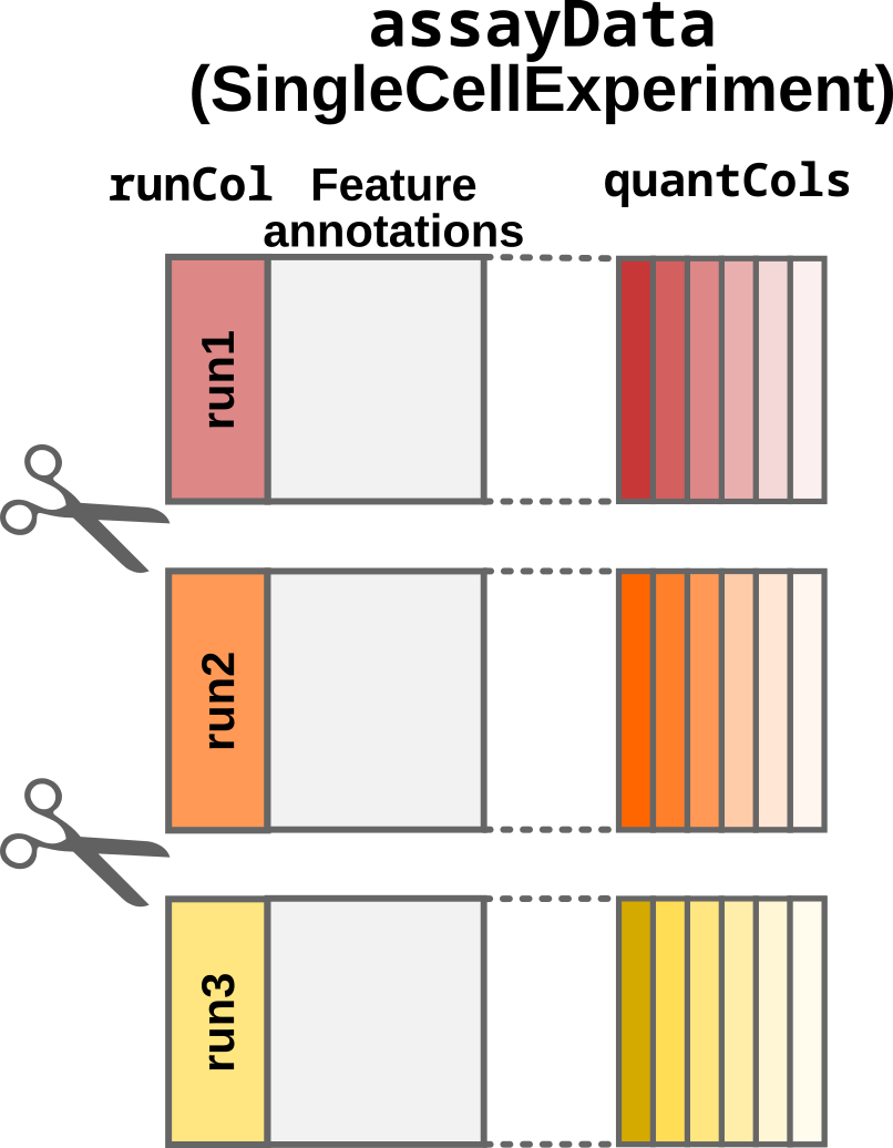
Step2: Split by acquisition run

The sample annotations are generated. If no colData is provided, the sample annotations are empty. Otherwise, readQFeatures() matches the information from assayData and colData based on quantCols (single-set case) or quantCols and runCol (multi-set case). Sample annotations are stored in the colData slot of the QFeatures object.

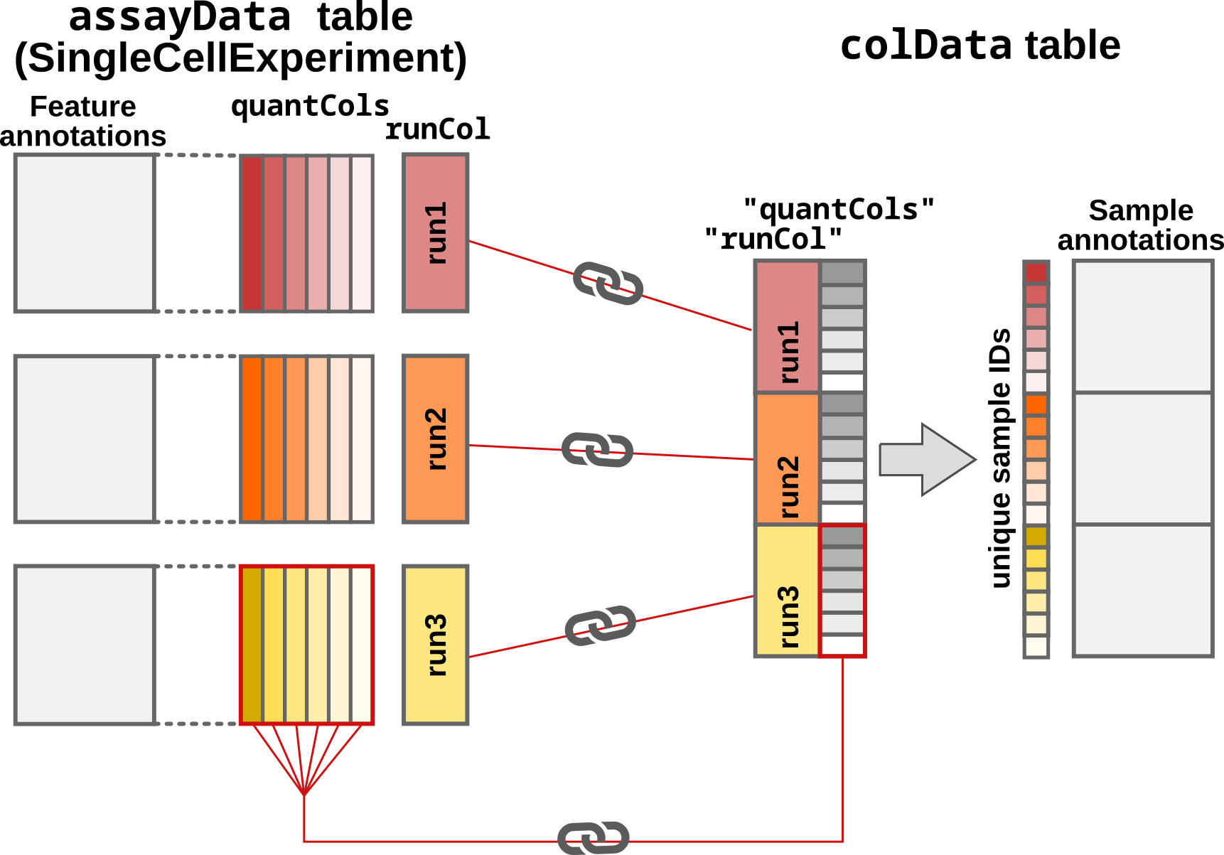
Step3: Adding and matching the sample annotations

Finally, the SummarizedExperiment sets and the colData are converted to a QFeatures object.

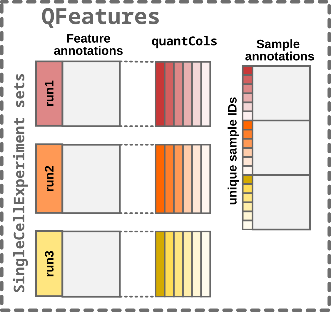
Step4: Converting to a QFeatures

What about other input formats?

readQFeatures() should work with any PSM quantification table that is output by a pre-processing software. For instance, you can easily import the PSM tables generated by Proteome Discoverer. The run names are contained in the File ID column (that should be supplied as the runCol argument to readQFeatures()). The quantification columns are contained in the columns starting with Abundance, eventually followed by a multiplexing tag name. These columns should be stored in a dedicated column in the colData data to be supplied as runCol to readQFeatures().

The QFeatures package is meant for both label-free and multiplexed proteomics data. Importing LFQ data is similar to the examples above with the only difference that quantCols would have only 1 element.

The readSCPfromDIANN() function is adapted to import label-free and plexDIA/mTRAQ Report.tsv files generated by DIA-NN.

For more information, see the ?readQFeatures() and ?readQFeaturesFromDIANN() manual pages, that described the main principle that concern the data import and formatting.

If your input cannot be loaded using the procedure described in this vignette, you can submit a feature request (see next section).

Need help?

You can open an issue on the GitHub repository in case of troubles when loading your data with readQFeatures(). Any suggestion or feature request about the function or the documentation are also warmly welcome.

Session information

R Under development (unstable) (2025-01-04 r87523)
Platform: x86_64-pc-linux-gnu
Running under: Ubuntu 24.04.1 LTS

Matrix products: default
BLAS:   /usr/lib/x86_64-linux-gnu/openblas-pthread/libblas.so.3 
LAPACK: /usr/lib/x86_64-linux-gnu/openblas-pthread/libopenblasp-r0.3.26.so;  LAPACK version 3.12.0

locale:
 [1] LC_CTYPE=en_US.UTF-8       LC_NUMERIC=C              
 [3] LC_TIME=en_US.UTF-8        LC_COLLATE=en_US.UTF-8    
 [5] LC_MONETARY=en_US.UTF-8    LC_MESSAGES=en_US.UTF-8   
 [7] LC_PAPER=en_US.UTF-8       LC_NAME=C                 
 [9] LC_ADDRESS=C               LC_TELEPHONE=C            
[11] LC_MEASUREMENT=en_US.UTF-8 LC_IDENTIFICATION=C       

time zone: UTC
tzcode source: system (glibc)

attached base packages:
[1] stats4    stats     graphics  grDevices utils     datasets  methods  
[8] base     

other attached packages:
 [1] DT_0.33                     QFeatures_1.17.2           
 [3] MultiAssayExperiment_1.33.4 SummarizedExperiment_1.37.0
 [5] Biobase_2.67.0              GenomicRanges_1.59.1       
 [7] GenomeInfoDb_1.43.2         IRanges_2.41.2             
 [9] S4Vectors_0.45.2            BiocGenerics_0.53.3        
[11] generics_0.1.3              MatrixGenerics_1.19.0      
[13] matrixStats_1.5.0           BiocStyle_2.35.0           

loaded via a namespace (and not attached):
 [1] xfun_0.50               bslib_0.8.0             htmlwidgets_1.6.4      
 [4] lattice_0.22-6          crosstalk_1.2.1         vctrs_0.6.5            
 [7] tools_4.5.0             tibble_3.2.1            cluster_2.1.8          
[10] pkgconfig_2.0.3         Matrix_1.7-1            desc_1.4.3             
[13] lifecycle_1.0.4         GenomeInfoDbData_1.2.13 compiler_4.5.0         
[16] stringr_1.5.1           textshaping_0.4.1       clue_0.3-66            
[19] htmltools_0.5.8.1       sass_0.4.9              yaml_2.3.10            
[22] lazyeval_0.2.2          pillar_1.10.1           pkgdown_2.1.1.9000     
[25] crayon_1.5.3            jquerylib_0.1.4         tidyr_1.3.1            
[28] MASS_7.3-64             DelayedArray_0.33.3     cachem_1.1.0           
[31] abind_1.4-8             tidyselect_1.2.1        digest_0.6.37          
[34] stringi_1.8.4           purrr_1.0.2             dplyr_1.1.4            
[37] reshape2_1.4.4          bookdown_0.42           fastmap_1.2.0          
[40] grid_4.5.0              cli_3.6.3               SparseArray_1.7.2      
[43] magrittr_2.0.3          S4Arrays_1.7.1          UCSC.utils_1.3.0       
[46] rmarkdown_2.29          XVector_0.47.2          httr_1.4.7             
[49] igraph_2.1.3            ragg_1.3.3              evaluate_1.0.1         
[52] knitr_1.49              rlang_1.1.4             Rcpp_1.0.13-1          
[55] glue_1.8.0              BiocManager_1.30.25     jsonlite_1.8.9         
[58] AnnotationFilter_1.31.0 R6_2.5.1                plyr_1.8.9             
[61] systemfonts_1.1.0       fs_1.6.5                ProtGenerics_1.39.1    
[64] MsCoreUtils_1.19.0

License

This vignette is distributed under a CC BY-SA license license.

Laurent Gatto

Christophe Vanderaa

10 January 2025

The `QFeatures` class

Converting tabular data

The single-set case

The multi-set case

Including sample annotations

Additional information

Sample names

Special case: empty samples

Reducing verbose

Under the hood

What about other input formats?

Need help?

Session information

License

Reference

Load mass spectrometry-based proteomics data using readQFeatures()

Laurent Gatto

Christophe Vanderaa

10 January 2025

The QFeatures class

Converting tabular data

The single-set case

The multi-set case

Including sample annotations

Additional information

Sample names

Special case: empty samples

Reducing verbose

Under the hood

What about other input formats?

Need help?

Session information

License

Reference

Load mass spectrometry-based proteomics data using `readQFeatures()`

The `QFeatures` class