#' R session:
install.packages("BiocManager")
BiocManager::install("SpectriPy")Detailed information on installation and configuration
Source:vignettes/detailed-installation-configuration.qmd
Introduction
This document provides detailed installation and configuration instructions for the SpectriPy package. For first time R users see also section Section 3.1 in the appendix. For advanced Python/system configuration and troubleshooting see sections Section 3.2 and Section 3.3 in the appendix.
Installation
SpectriPy relies on, and extends, the reticulate package for interoperability between Python and R. For installation of SpectriPy, Python needs to be installed on the system. See also the Install Python Packages documentation from the reticulate package for information on installing Python. Since version 0.99.5, SpectriPy uses the new py_require() function from the reticulate package to install and manage all required Python libraries (i.e., matchms, spectrum_utils and numpy) including all their dependencies.
Installation of the package using:
should work on most systems. See also section Fixing package installation or loading problems in the appendix of the SpectriPy vignette if installing or loading of the package fails.
Configure reticulate with host system Python environment (optional)
SpectriPy (respectively reticulate) can be configured to use an available Python environment of the host system, instead of using the automatic setup. In this case, however, the user must first install the required Python libraries manually in that local environment. The required libraries are:
- matchms 0.31
- spectrum_utils 0.3.2
- numpy 2.2.0
To use SpectriPy with a local, system, Python environment either the RETICULATE_PYTHON or the RETICULATE_PYTHON_ENV environment variable needs to be set. The former should point to the python binary, while the latter should point to the (virtualenv or conda) environment with all necessary libraries installed. These environment variables can either be set globally in the operation system settings, or specifically for R. See also the Environment documentation from Posit for more information on how to define environment variables for R. In the example below, we set the variable using Sys.setenv() before the SpectriPy or reticulate libraries are loaded:
#' R session:

Sys.setenv(RETICULATE_PYTHON_ENV="<path-to-the-virtualenv-with-libraries>")
library(SpectriPy)
The Sys.setenv() call can also be added to a .Rprofile file to automatically set the environmental variable when R starts.
SpectriPy pre-requisites and installation instructions
Installing Bioconductor
Bioconductor is required to install SpectriPy, as described below and from source https://bioconductor.org/install/.
The current release of Bioconductor is version 3.21; it works with R version 4.5.0. Users of older R and Bioconductor must update their installation to take advantage of new features and to access packages that have been added to Bioconductor since the last release.
The development version of Bioconductor is version 3.22; it works with R version 4.5.0. More recent devel versions of R (if available) will be supported during the next Bioconductor release cycle.
Once R has been installed, get the latest version of Bioconductor by starting R and entering the following commands.
It may be possible to change the Bioconductor version of an existing installation; see the Changing version section of the BiocManager vignette.
Details, including instructions to install additional packages and to update, find, and troubleshoot are provided below. A devel version of Bioconductor is available. There are good reasons for using BiocManager::install() for managing Bioconductor resources.
#' R session:

if (!require("BiocManager", quietly = TRUE))
    install.packages("BiocManager")
BiocManager::install(version = "3.21")
Installing SpectriPy
SpectriPy can be installed through Bioconductor:
#' R session:

BiocManager::install("SpectriPy")
Check installation completed
The status of installation can be easily checked by starting R and entering the following commands.
This command loads the SpectriPy package, if correct installed. py_availble() should return TRUE.
Appendix
Installation instructions for first-time R users
Instructions to install R and RStudio for the first time are described below, from source https://rstudio-education.github.io/hopr/packages2.html.
Installing R and RStudio
To get started with R, you need to acquire your own copy. This appendix will show you how to download R as well as RStudio, a software application that makes R easier to use. You’ll go from downloading R to opening your first R session.
Both R and RStudio are free and easy to download.
How to Download and Install R
R is maintained by an international team of developers who make the language available through the web page of The Comprehensive R Archive Network. The top of the web page provides three links for downloading R. Follow the link that describes your operating system: Windows, Mac, or Linux.
Windows
To install R on Windows, click the “Download R for Windows” link. Then click the base link. Next, click the first link at the top of the new page. This link should say something like Download R 3.0.3 for Windows, except the 3.0.3 will be replaced by the most current version of R. The link downloads an installer program, which installs the most up-to-date version of R for Windows. Run this program and step through the installation wizard that appears. The wizard will install R into your program files folders and place a shortcut in your Start menu. Note that you’ll need to have all of the appropriate administration privileges to install new software on your machine.
Mac
To install R on a Mac, click the Download R for Mac link. Next, click on the R-3.0.3 package link (or the package link for the most current release of R). An installer will download to guide you through the installation process, which is very easy. The installer lets you customize your installation, but the defaults will be suitable for most users. I’ve never found a reason to change them. If your computer requires a password before installing new progams, you’ll need it here.
Binaries Versus Source
R can be installed from precompiled binaries or built from source on any operating system. For Windows and Mac machines, installing R from binaries is extremely easy. The binary comes preloaded in its own installer. Although you can build R from source on these platforms, the process is much more complicated and won’t provide much benefit for most users. For Linux systems, the opposite is true. Precompiled binaries can be found for some systems, but it is much more common to build R from source files when installing on Linux. The download pages on CRAN’s website provide information about building R from source for the Windows, Mac, and Linux platforms.
Linux
R comes preinstalled on many Linux systems, but you’ll want the newest version of R if yours is out of date. The CRAN website provides files to build R from source on Debian, Redhat, SUSE, and Ubuntu systems under the link Download R for Linux. Click the link and then follow the directory trail to the version of Linux you wish to install on. The exact installation procedure will vary depending on the Linux system you use. CRAN guides the process by grouping each set of source files with documentation or README files that explain how to install on your system.
32-bit Versus 64-bit
R comes in both 32-bit and 64-bit versions. Which should you use? In most cases, it won’t matter. Both versions use 32-bit integers, which means they compute numbers to the same numerical precision. The difference occurs in the way each version manages memory. 64-bit R uses 64-bit memory pointers, and 32-bit R uses 32-bit memory pointers. This means 64-bit R has a larger memory space to use (and search through). As a rule of thumb, 32-bit builds of R are faster than 64-bit builds, though not always. On the other hand, 64-bit builds can handle larger files and data sets with fewer memory management problems. In either version, the maximum allowable vector size tops out at around 2 billion elements. If your operating system doesn’t support 64-bit programs, or your RAM is less than 4 GB, 32-bit R is for you. The Windows and Mac installers will automatically install both versions if your system supports 64-bit R.
Using R
R isn’t a program that you can open and start using, like Microsoft Word or Internet Explorer. Instead, R is a computer language, like C, C++, or UNIX. You use R by writing commands in the R language and asking your computer to interpret them. In the old days, people ran R code in a UNIX terminal window—as if they were hackers in a movie from the 1980s. Now almost everyone uses R with an application called RStudio, and I recommend that you do, too.
R and UNIX
You can still run R in a UNIX or BASH window by typing the command:
Rwhich opens an R interpreter. You can then do your work and close the interpreter by running q() when you are finished.
RStudio
RStudio is an application like Microsoft Word—except that instead of helping you write in English, RStudio helps you write in R. I use RStudio throughout the book because it makes using R much easier. Also, the RStudio interface looks the same for Windows, Mac OS, and Linux. That will help me match the book to your personal experience.
You can download RStudio for free. Just click the Download RStudio button and follow the simple instructions that follow. Once you’ve installed RStudio, you can open it like any other program on your computer—usually by clicking an icon on your desktop.
The R GUIs
Windows and Mac users usually do not program from a terminal window, so the Windows and Mac downloads for R come with a simple program that opens a terminal-like window for you to run R code in. This is what opens when you click the R icon on your Windows or Mac computer. These programs do a little more than the basic terminal window, but not much. You may hear people refer to them as the Windows or Mac R GUIs.
When you open RStudio, a window appears with three panes in it, as in Figure 1. The largest pane is a console window. This is where you’ll run your R code and see results. The console window is exactly what you’d see if you ran R from a UNIX console or the Windows or Mac GUIs. Everything else you see is unique to RStudio. Hidden in the other panes are a text editor, a graphics window, a debugger, a file manager, and much more. You’ll learn about these panes as they become useful throughout the course of this book. The RStudio IDE for R.
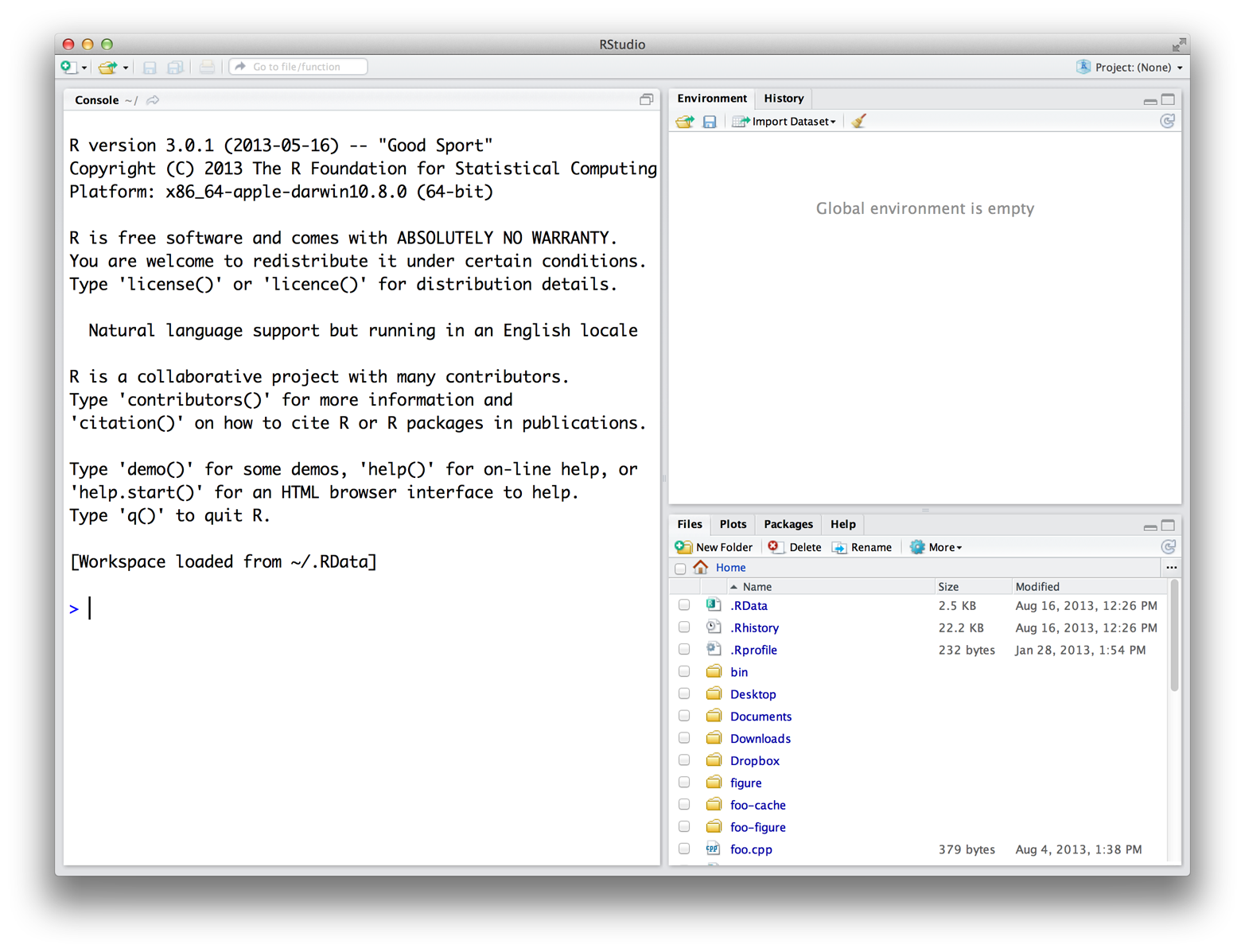
Figure 1: The RStudio IDE for R.
Do I still need to download R?
Even if you use RStudio, you’ll still need to download R to your computer. RStudio helps you use the version of R that lives on your computer, but it doesn’t come with a version of R on its own.
Opening R
Now that you have both R and RStudio on your computer, you can begin using R by opening the RStudio program. Open RStudio just as you would any program, by clicking on its icon or by typing RStudio at the Windows Run prompt.
Startup and Python configuration
The way Python dependencies are defined and managed has changed in SpectriPy beginning with version 0.99.6. SpectriPy now declares Python dependencies using the py_require() function from the reticulate package. These Python package dependencies requested via py_require() will automatically be provisioned and made available for the user when the SpectriPy package is loaded, via an ephemeral Python virtual environment. Eventually missing libraries are downloaded and installed automatically.
The previous virtualenv or conda-based setup is now replaced by the preferred py_require() approach, hence the previous package’s options and environment variables "spectripy.use_system", SPECTRIPY_USE_SYSTEM, "spectripy.use_conda", SPECTRIPY_USE_CONDA, "spectripy.env", SPECTRIPY_ENV are now ignored.
A pre-defined Python environment can be used by pointing the RETICULATE_PYTHON environment variable to the respective Python binary or the RETICULATE_PYTHON_ENV to the path of the environment. All Python libraries required by SpectriPy need however to be installed and available in that Python environment, as SpectriPy respectively reticulate’s py_require() functionality will be bypassed. These Python libraries are:
- matchms >= 0.31
- spectrum_utils >= 0.3.2
- numpy >= 2.2.0
More information on this manual setup can be found in the Detailed information on installation and configuration vignette.
See also the help of the reticulate package for more information on configuring Python with R.
Fixing package installation or loading problems
SpectriPy loads and imports the required Python libraries matchms, spectrum_utils and numpy during package loading/attaching (e.g. using library(SpectriPy)). Installation or loading of the package can thus fail if these libraries or the required versions can not be found. SpectriPy uses the newer py_require() approach from the reticulate package to manage Python requirements.
Trouble shooting:
Check the output of
Sys.getenv(): is there a system variableRETICULATE_PYTHONorRETICULATE_PYTHON_ENVdefined? Problem: reticulate will use the specified Python or Python environment and skip automatic installation of the Python libraries. Solution: a) unset this environment variables b) manually install the required Python libraries in that Python environment (see section Section 3.2).Is there a default r-reticulate virtual environment (e.g. created by another package or a previous version of reticulate) on the system, i.e., does
virtualenv_exists("r-reticulate")returnTRUE? Problem: reticulate will use this environment instead of the ephemeral virtual environment that would be managed throughpy_require(). Solution: define an environment variableRETICULATE_USE_MANAGED_VENV="yes". This variable can either be defined system wide, or by adding a lineRETICULATE_USE_MANAGED_VENV="yes"to a file named .Renviron in the user’s home directory. See also the Environment documentation from Posit for more information on how to define environment variables for R.
If this does not solve the issue, have also a look at the order of discovery documentation of reticulate which clearly explains how reticulate tries to define and use the Python setup. Most SpectriPy installation/loading problems come from the fact that another Python setup than the ephemeral virtual environment (which is the current suggested mode) is used. The solution suggested in point 2 above should solve most of these problems.
More information can also be found in the reticulate’s Python version configuration documentation.
Session information
#' R session:

sessionInfo()
R version 4.6.0 (2026-04-24)
Platform: x86_64-pc-linux-gnu
Running under: Ubuntu 24.04.4 LTS
Matrix products: default
BLAS: /usr/lib/x86_64-linux-gnu/openblas-pthread/libblas.so.3
LAPACK: /usr/lib/x86_64-linux-gnu/openblas-pthread/libopenblasp-r0.3.26.so; LAPACK version 3.12.0
locale:
[1] LC_CTYPE=en_US.UTF-8 LC_NUMERIC=C
[3] LC_TIME=en_US.UTF-8 LC_COLLATE=en_US.UTF-8
[5] LC_MONETARY=en_US.UTF-8 LC_MESSAGES=en_US.UTF-8
[7] LC_PAPER=en_US.UTF-8 LC_NAME=C
[9] LC_ADDRESS=C LC_TELEPHONE=C
[11] LC_MEASUREMENT=en_US.UTF-8 LC_IDENTIFICATION=C
time zone: UTC
tzcode source: system (glibc)
attached base packages:
[1] stats graphics grDevices utils datasets methods base
other attached packages:
[1] SpectriPy_1.3.0 reticulate_1.46.0
loaded via a namespace (and not attached):
[1] Spectra_1.23.0 cli_3.6.6 knitr_1.51
[4] rlang_1.2.0 xfun_0.57 ProtGenerics_1.45.0
[7] otel_0.2.0 png_0.1-9 generics_0.1.4
[10] data.table_1.18.4 jsonlite_2.0.0 clue_0.3-68
[13] S4Vectors_0.51.1 htmltools_0.5.9 stats4_4.6.0
[16] rmarkdown_2.31 grid_4.6.0 snakecase_0.11.1
[19] evaluate_1.0.5 MASS_7.3-65 fastmap_1.2.0
[22] yaml_2.3.12 IRanges_2.47.0 MsCoreUtils_1.25.3
[25] cluster_2.1.8.2 compiler_4.6.0 codetools_0.2-20
[28] fs_2.1.0 Rcpp_1.1.1-1.1 MetaboCoreUtils_1.21.1
[31] BiocParallel_1.47.0 lattice_0.22-9 digest_0.6.39
[34] parallel_4.6.0 Matrix_1.7-5 withr_3.0.2
[37] tools_4.6.0 BiocGenerics_0.59.0