install.packages("BiocManager")
BiocManager::install("SpectriPy")Enabling integration of Python libraries and R packages for combined mass spectrometry data analysis
Source:vignettes/SpectriPy.qmd
Compiled: Tue May 12 06:50:00 2026
Note: since version 0.99.6 SpectriPy uses the newer, recommended approach to install and configure required Python libraries (i.e., through reticulate’s py_require() functionality). This affects also the way a pre-defined Python environment can be used. See section Startup and Python configuration in the Detailed information on installation and configuration vignette for updated information.
Introduction
Powerful software libraries for mass spectrometry (MS) data are available in both Python and R, covering specific and sometimes distinct aspects in the analysis of proteomics and metabolomics data. R’s reticulate package converts basic data types between Python and R and enables a seamless interoperability of both programming languages. The SpectriPy package extends reticulate allowing to translate MS data data structures between R and Python, specifically, between R’s Spectra objects and Python MS data structures from the matchms and spectrum_utils Python libraries. In addition, functionality from Python’s matchms library is directly wrapped into R functions allowing a seamless integration into R based workflows. SpectriPy thus enables powerful proteomics or metabolomics analysis workflows combining the strengths of Python and R MS libraries.
This vignette provides information on how to share and translate MS data structures between R and Python to enable combined Python and R-based analysis workflows. For an example use case analysis, see the SpectriPy tutorial: Annotation of LC-MS/MS spectra vignette.
System requirements
The reticulate package enables a seamless integration of Python with R by translating the core data structures between the two programming languages and sharing a Python (respectively R) runtime environment, including shared variables, that can be accessed from the other programming language. If the reticulate package is not already available, it will be installed during the installation of SpectriPy. Alternatively, it can be installed using install.packages("reticulate").
The SpectriPy package builds on reticulate providing in addition the functionality to translate data structures for MS data between the two languages. Specifically, the package translates between R’s Spectra objects (from the Spectra package) and Python’s matchms.Spectrum and spectrum_utils.spectrum.MsmsSpectrum objects from the matchms and spectrum_utils Python libraries, respectively.
Installation
If the BiocManager package is not already available, please install it with install.packages("BiocManager"). As a system dependency, the package requires Python (version >= 3.12) to be available. During package installation, SpectriPy will by default install all required Python libraries automatically. See section Startup and Python configuration in the Detailed information on installation and configuration vignette for information on manual library installation or usage of a pre-defined or system Python environment. See section Fixing package installation or loading problems in the Detailed information on installation and configuration vignette for some hints how to solve package installation or loading problems.
To install the package use the code below:
Translating data structures between R and Python
This section describes how MS data is being converted between R and Python to enable analyses combining both programming/analysis languages and accessing the same shared MS data. The first two sections describe how MS data can be converted between R and Python. See also section Section 4.4 for a more elegant approach and improved integration with Spectra-based workflows in R.
Library loading and system setup
Below we load all required packages. By loading SpectriPy, the package will evaluate if the required Python libraries (i.e., matchms version >= 0.1, spectrum_utils version >= 0.3.2 and numpy version >= 2.2) are available. If they are not available, SpectriPy will install them using functionality from the reticulate R package. See section Startup and Python configuration in the Detailed information on installation and configuration vignette for more configuration options of SpectriPy.
The reticulate package will be loaded by SpectriPy, ensuring the R/Python integration provided by that package to be available as well. To better discriminate between R and Python code chunks, we add the comment #' R session: or #' Python session: to label the R and Python code chunks, respectively.
Converting MS data from R to Python
In this section we show how MS data can be converted from R to Python. Below we first define the name and path of a data file in mzML format (provided by the r BiocStyle::Biocpkg("MsDataHub") package) and load that data as an R Spectra object. We thus first ensure that the package MsDataHub is installed. If the line below results in an error you need to first install MsDataHub using BiocManager::install("MsDataHub").
Loading required package: MsDataHubNext, we define the file path to the test file and load the data as a Spectra object in R.
#' R session:

#' Loading the data from a mzML file as a `Spectra` object
library(MsDataHub)
fl <- MsDataHub::PestMix1_DDA.mzML()
mzml_r <- Spectra(fl)
We next restrict the data to MS level 2 and remove spectra with less than 3 (fragment) peaks.
#' R session:

#' Restrict to MS level 2 spectra
mzml_r <- filterMsLevel(mzml_r, 2)
mzml_r <- mzml_r[lengths(mzml_r) >= 3]
mzml_r
MSn data (Spectra) with 2243 spectra in a MsBackendMzR backend:
msLevel rtime scanIndex
<integer> <numeric> <integer>
1 2 7.216 58
2 2 13.146 106
3 2 13.556 108
4 2 23.085 186
5 2 27.385 219
... ... ... ...
2239 2 894.762 7566
2240 2 895.182 7568
2241 2 895.472 7570
2242 2 896.252 7575
2243 2 898.602 7591
... 34 more variables/columns.
file(s):
431539cd57e_7861
Processing:
Filter: select MS level(s) 2 [Tue May 12 06:50:17 2026] This Spectra object can now be converted to equivalent data structures in Python using the rspec_to_pyspec() function:
#' R session:

#' Convert the R Spectra to a list of Python matchms.Spectrum objects
tmp <- rspec_to_pyspec(mzml_r)
The tmp variable is now a Python list of matchms.Spectrum objects:
#' R session:

#' Class of the converted variable
class(tmp)
[1] "python.builtin.list" "python.builtin.object"
#' First element
class(tmp[1])
[1] "matchms.Spectrum.Spectrum" "python.builtin.object" Note that this Python data structure is now stored within the R session. Therefore, we have two full copies of the data in memory, i.e., an R Spectra object and a Python matchms.Spectrum object (see Section Section 4.4 for an alternative to avoid multiple data copies). We can access the variable from the associated Python environment through reticulate’s special r attribute using r.<variable name in R>.
#' Python session:

#' Access the Python data structure stored in the R session
r.tmp
[Spectrum(precursor m/z=137.96, 3 fragments between 55.9 and 138.0), Spectrum(precursor m/z=56.94, 3 fragments between 55.9 and 57.0), Spectrum(precursor m/z=89.94, 3 fragments between 53.9 and 72.9), Spectrum(precursor m/z=207.03, 3 fragments between 130.9 and 191.0), Spectrum(precursor m/z=121.10, 11 fragments between 51.0 and 121.1), Spectrum(precursor m/z=429.09, 8 fragments between 73.0 and 341.0), Spectrum(precursor m/z=121.04, 7 fragments between 51.0 and 121.0), Spectrum(precursor m/z=55.01, 4 fragments between 54.9 and 55.0), Spectrum(precursor m/z=81.07, 3 fragments between 53.0 and 81.1), Spectrum(precursor m/z=55.93, 4 fragments between 55.9 and 57.0), Spectrum(precursor m/z=80.05, 16 fragments between 50.0 and 241.2), Spectrum(precursor m/z=80.05, 5 fragments between 50.0 and 80.1), Spectrum(precursor m/z=74.10, 3 fragments between 74.1 and 74.1), Spectrum(precursor m/z=80.05, 11 fragments between 50.0 and 384.9), Spectrum(precursor m/z=258.89, 4 fragments between 101.1 and 173.9), Spectrum(precursor m/z=142.96, 15 fragments between 55.9 and 130.0), Spectrum(precursor m/z=172.98, 28 fragments between 51.9 and 173.1), Spectrum(precursor m/z=126.97, 24 fragments between 53.0 and 243.1), Spectrum(precursor m/z=194.12, 12 fragments between 55.9 and 194.1), Spectrum(precursor m/z=217.12, 26 fragments between 55.0 and 217.1), Spectrum(precursor m/z=97.97, 4 fragments between 54.9 and 81.9), Spectrum(precursor m/z=208.94, 8 fragments between 132.9 and 209.1), Spectrum(precursor m/z=135.04, 11 fragments between 51.0 and 135.0), Spectrum(precursor m/z=467.87, 22 fragments between 145.0 and 413.8), Spectrum(precursor m/z=224.13, 21 fragments between 51.0 and 224.1), Spectrum(precursor m/z=113.96, 16 fragments between 51.0 and 114.1), Spectrum(precursor m/z=126.03, 10 fragments between 64.0 and 127.0), Spectrum(precursor m/z=104.01, 3 fragments between 57.9 and 78.0), Spectrum(precursor m/z=194.12, 14 fragments between 58.1 and 1108.8), Spectrum(precursor m/z=113.96, 9 fragments between 55.0 and 114.1), Spectrum(precursor m/z=194.12, 8 fragments between 51.0 and 194.1), Spectrum(precursor m/z=156.97, 4 fragments between 53.9 and 70.9), Spectrum(precursor m/z=194.12, 6 fragments between 55.9 and 194.1), Spectrum(precursor m/z=55.04, 21 fragments between 54.0 and 244.6), Spectrum(precursor m/z=74.06, 3 fragments between 57.0 and 74.1), Spectrum(precursor m/z=142.99, 33 fragments between 55.1 and 242.5), Spectrum(precursor m/z=74.06, 5 fragments between 57.0 and 74.1), Spectrum(precursor m/z=142.99, 20 fragments between 51.9 and 143.0), Spectrum(precursor m/z=75.03, 4 fragments between 55.9 and 57.0), Spectrum(precursor m/z=179.10, 11 fragments between 51.9 and 179.1), Spectrum(precursor m/z=127.04, 17 fragments between 51.0 and 127.0), Spectrum(precursor m/z=112.01, 6 fragments between 53.9 and 460.4), Spectrum(precursor m/z=142.01, 25 fragments between 51.0 and 142.0), Spectrum(precursor m/z=142.01, 24 fragments between 55.1 and 143.0), Spectrum(precursor m/z=112.01, 6 fragments between 55.9 and 112.0), Spectrum(precursor m/z=142.01, 23 fragments between 55.9 and 143.0), Spectrum(precursor m/z=112.02, 7 fragments between 53.9 and 112.0), Spectrum(precursor m/z=124.98, 8 fragments between 55.1 and 883.7), Spectrum(precursor m/z=124.98, 3 fragments between 55.9 and 79.0), Spectrum(precursor m/z=367.97, 4 fragments between 227.0 and 368.0), Spectrum(precursor m/z=508.98, 11 fragments between 134.0 and 368.0), Spectrum(precursor m/z=163.99, 3 fragments between 55.9 and 135.1), Spectrum(precursor m/z=399.92, 36 fragments between 57.0 and 336.9), Spectrum(precursor m/z=367.97, 7 fragments between 134.0 and 305.0), Spectrum(precursor m/z=508.98, 13 fragments between 179.0 and 368.0), Spectrum(precursor m/z=229.98, 3 fragments between 108.0 and 168.0), Spectrum(precursor m/z=241.93, 5 fragments between 94.0 and 151.9), Spectrum(precursor m/z=399.92, 19 fragments between 136.9 and 336.9), Spectrum(precursor m/z=508.97, 13 fragments between 135.0 and 368.0), Spectrum(precursor m/z=524.95, 11 fragments between 149.9 and 384.0), Spectrum(precursor m/z=241.93, 4 fragments between 94.0 and 181.9), Spectrum(precursor m/z=382.93, 5 fragments between 197.9 and 288.9), Spectrum(precursor m/z=399.93, 51 fragments between 118.9 and 399.9), Spectrum(precursor m/z=112.02, 6 fragments between 55.9 and 95.0), Spectrum(precursor m/z=197.94, 3 fragments between 53.9 and 139.0), Spectrum(precursor m/z=241.93, 9 fragments between 134.9 and 209.9), Spectrum(precursor m/z=383.95, 5 fragments between 102.0 and 243.0), Spectrum(precursor m/z=524.96, 6 fragments between 149.9 and 384.0), Spectrum(precursor m/z=142.01, 64 fragments between 55.1 and 143.0), Spectrum(precursor m/z=231.48, 4 fragments between 71.0 and 150.0), Spectrum(precursor m/z=524.95, 12 fragments between 149.0 and 384.0), Spectrum(precursor m/z=142.01, 30 fragments between 51.0 and 143.0), Spectrum(precursor m/z=225.96, 3 fragments between 85.0 and 118.9), Spectrum(precursor m/z=383.95, 10 fragments between 101.9 and 337.9), Spectrum(precursor m/z=126.98, 12 fragments between 51.9 and 127.0), Spectrum(precursor m/z=163.99, 3 fragments between 55.9 and 120.1), Spectrum(precursor m/z=367.98, 5 fragments between 132.0 and 305.0), Spectrum(precursor m/z=508.98, 21 fragments between 132.0 and 369.0), Spectrum(precursor m/z=104.01, 19 fragments between 60.1 and 245.0), Spectrum(precursor m/z=445.12, 25 fragments between 73.0 and 429.1), Spectrum(precursor m/z=141.96, 47 fragments between 55.8 and 143.0), Spectrum(precursor m/z=141.96, 30 fragments between 55.9 and 142.0), Spectrum(precursor m/z=429.09, 8 fragments between 75.0 and 429.1), Spectrum(precursor m/z=55.01, 5 fragments between 54.0 and 923.4), Spectrum(precursor m/z=56.05, 15 fragments between 55.9 and 245.0), Spectrum(precursor m/z=281.05, 13 fragments between 73.0 and 281.1), Spectrum(precursor m/z=327.08, 20 fragments between 63.0 and 327.1), Spectrum(precursor m/z=55.01, 3 fragments between 54.0 and 55.0), Spectrum(precursor m/z=142.99, 26 fragments between 55.1 and 243.0), Spectrum(precursor m/z=206.00, 5 fragments between 71.9 and 206.0), Spectrum(precursor m/z=206.00, 6 fragments between 64.0 and 268.9), Spectrum(precursor m/z=124.98, 6 fragments between 55.9 and 79.0), Spectrum(precursor m/z=190.03, 8 fragments between 85.0 and 176.9), Spectrum(precursor m/z=144.99, 12 fragments between 51.0 and 145.0), Spectrum(precursor m/z=373.04, 6 fragments between 73.0 and 267.0), Spectrum(precursor m/z=142.99, 16 fragments between 61.0 and 143.0), Spectrum(precursor m/z=184.02, 14 fragments between 57.9 and 143.0), Spectrum(precursor m/z=267.97, 3 fragments between 102.9 and 150.9), Spectrum(precursor m/z=389.01, 5 fragments between 64.0 and 258.9), Spectrum(precursor m/z=113.00, 5 fragments between 55.9 and 95.0), Spectrum(precursor m/z=142.99, 40 fragments between 51.6 and 143.0), Spectrum(precursor m/z=420.95, 17 fragments between 144.0 and 420.9), Spectrum(precursor m/z=124.98, 4 fragments between 55.9 and 79.0), Spectrum(precursor m/z=184.02, 29 fragments between 56.9 and 151.9), Spectrum(precursor m/z=390.99, 19 fragments between 64.0 and 391.0), Spectrum(precursor m/z=373.04, 6 fragments between 101.0 and 267.0), Spectrum(precursor m/z=420.95, 6 fragments between 118.9 and 379.9), Spectrum(precursor m/z=467.97, 5 fragments between 222.0 and 405.0), Spectrum(precursor m/z=587.99, 16 fragments between 165.0 and 405.0), Spectrum(precursor m/z=142.99, 29 fragments between 61.0 and 143.0), Spectrum(precursor m/z=184.02, 14 fragments between 64.0 and 143.0), Spectrum(precursor m/z=202.99, 8 fragments between 71.0 and 274.9), Spectrum(precursor m/z=206.00, 3 fragments between 64.0 and 206.0), Spectrum(precursor m/z=267.97, 3 fragments between 102.9 and 222.0), Spectrum(precursor m/z=390.99, 8 fragments between 149.0 and 391.0), Spectrum(precursor m/z=420.95, 8 fragments between 144.0 and 421.0), Spectrum(precursor m/z=294.50, 13 fragments between 118.9 and 274.9), Spectrum(precursor m/z=373.04, 4 fragments between 73.0 and 190.0), Spectrum(precursor m/z=467.97, 13 fragments between 165.0 and 405.0), Spectrum(precursor m/z=94.99, 4 fragments between 51.0 and 288.6), Spectrum(precursor m/z=404.98, 19 fragments between 135.0 and 1949.3), Spectrum(precursor m/z=55.01, 4 fragments between 54.0 and 55.0), Spectrum(precursor m/z=113.00, 9 fragments between 53.9 and 113.0), Spectrum(precursor m/z=239.09, 6 fragments between 83.1 and 239.1), Spectrum(precursor m/z=127.04, 12 fragments between 51.9 and 127.0), Spectrum(precursor m/z=114.10, 8 fragments between 51.9 and 114.1), Spectrum(precursor m/z=139.96, 10 fragments between 53.9 and 366.9), Spectrum(precursor m/z=610.18, 11 fragments between 147.1 and 610.2), Spectrum(precursor m/z=239.15, 9 fragments between 51.9 and 239.1), Spectrum(precursor m/z=198.18, 11 fragments between 51.9 and 198.2), Spectrum(precursor m/z=89.51, 5 fragments between 55.9 and 123.0), Spectrum(precursor m/z=428.89, 7 fragments between 73.0 and 341.0), Spectrum(precursor m/z=52.02, 3 fragments between 51.0 and 114.6), Spectrum(precursor m/z=198.18, 15 fragments between 53.0 and 198.2), Spectrum(precursor m/z=79.00, 4 fragments between 50.0 and 66.0), Spectrum(precursor m/z=130.16, 4 fragments between 57.1 and 130.2), Spectrum(precursor m/z=56.05, 3 fragments between 55.9 and 56.0), Spectrum(precursor m/z=279.08, 21 fragments between 57.1 and 279.1), Spectrum(precursor m/z=156.02, 4 fragments between 52.9 and 125.0), Spectrum(precursor m/z=283.17, 10 fragments between 55.1 and 283.2), Spectrum(precursor m/z=55.04, 3 fragments between 54.0 and 55.0), Spectrum(precursor m/z=283.17, 6 fragments between 69.1 and 251.0), Spectrum(precursor m/z=305.16, 6 fragments between 129.9 and 305.2), Spectrum(precursor m/z=124.97, 4 fragments between 55.9 and 79.0), Spectrum(precursor m/z=300.20, 8 fragments between 89.1 and 283.2), Spectrum(precursor m/z=174.99, 18 fragments between 53.9 and 690.8), Spectrum(precursor m/z=446.12, 27 fragments between 73.0 and 342.0), Spectrum(precursor m/z=130.16, 7 fragments between 61.0 and 130.1), Spectrum(precursor m/z=119.08, 10 fragments between 51.0 and 119.1), Spectrum(precursor m/z=113.96, 36 fragments between 51.0 and 244.3), Spectrum(precursor m/z=96.96, 11 fragments between 51.0 and 81.9), Spectrum(precursor m/z=327.20, 28 fragments between 51.0 and 327.1), Spectrum(precursor m/z=327.20, 10 fragments between 77.0 and 327.2), Spectrum(precursor m/z=344.23, 6 fragments between 89.1 and 344.2), Spectrum(precursor m/z=137.96, 4 fragments between 53.0 and 102.0), Spectrum(precursor m/z=344.23, 9 fragments between 87.0 and 327.2), Spectrum(precursor m/z=157.01, 8 fragments between 74.9 and 157.0), Spectrum(precursor m/z=198.18, 8 fragments between 53.9 and 198.2), Spectrum(precursor m/z=157.01, 18 fragments between 53.9 and 157.0), Spectrum(precursor m/z=157.01, 10 fragments between 55.1 and 157.0), Spectrum(precursor m/z=198.18, 16 fragments between 53.9 and 198.2), Spectrum(precursor m/z=127.01, 18 fragments between 51.9 and 172.4), Spectrum(precursor m/z=89.50, 9 fragments between 54.9 and 137.9), Spectrum(precursor m/z=56.01, 4 fragments between 55.9 and 56.1), Spectrum(precursor m/z=327.01, 18 fragments between 63.0 and 327.1), Spectrum(precursor m/z=130.97, 12 fragments between 54.9 and 113.0), Spectrum(precursor m/z=388.25, 18 fragments between 57.1 and 388.3), Spectrum(precursor m/z=89.94, 11 fragments between 54.9 and 1050.3), Spectrum(precursor m/z=84.00, 23 fragments between 236.6 and 244.7), Spectrum(precursor m/z=371.22, 18 fragments between 55.1 and 355.1), Spectrum(precursor m/z=388.25, 6 fragments between 87.0 and 371.2), Spectrum(precursor m/z=89.51, 7 fragments between 55.9 and 109.9), Spectrum(precursor m/z=83.00, 8 fragments between 51.0 and 84.1), Spectrum(precursor m/z=219.09, 19 fragments between 56.9 and 219.1), Spectrum(precursor m/z=80.05, 4 fragments between 51.0 and 80.1), Spectrum(precursor m/z=116.11, 9 fragments between 55.0 and 116.1), Spectrum(precursor m/z=116.11, 30 fragments between 53.0 and 116.1), Spectrum(precursor m/z=116.11, 39 fragments between 53.0 and 116.1), Spectrum(precursor m/z=154.96, 9 fragments between 51.9 and 155.1), Spectrum(precursor m/z=432.28, 8 fragments between 87.0 and 432.3), Spectrum(precursor m/z=432.28, 11 fragments between 89.1 and 432.3), Spectrum(precursor m/z=432.28, 8 fragments between 89.1 and 432.3), Spectrum(precursor m/z=56.05, 4 fragments between 55.9 and 57.0), Spectrum(precursor m/z=331.00, 8 fragments between 63.0 and 331.0), Spectrum(precursor m/z=429.08, 8 fragments between 75.0 and 341.0), Spectrum(precursor m/z=233.07, 24 fragments between 91.1 and 782.5), Spectrum(precursor m/z=476.30, 16 fragments between 73.1 and 1214.6), Spectrum(precursor m/z=459.27, 4 fragments between 89.1 and 459.3), Spectrum(precursor m/z=476.30, 9 fragments between 87.0 and 476.3), Spectrum(precursor m/z=476.30, 19 fragments between 89.1 and 476.3), Spectrum(precursor m/z=55.01, 5 fragments between 54.0 and 55.0), Spectrum(precursor m/z=333.19, 18 fragments between 99.0 and 333.2), Spectrum(precursor m/z=520.33, 19 fragments between 87.0 and 520.3), Spectrum(precursor m/z=520.33, 19 fragments between 73.0 and 521.4), Spectrum(precursor m/z=130.12, 20 fragments between 51.0 and 130.2), Spectrum(precursor m/z=130.12, 25 fragments between 53.9 and 130.1), Spectrum(precursor m/z=130.12, 19 fragments between 55.0 and 130.1), Spectrum(precursor m/z=182.19, 29 fragments between 53.0 and 245.0), Spectrum(precursor m/z=182.19, 20 fragments between 53.0 and 182.2), Spectrum(precursor m/z=182.19, 12 fragments between 54.9 and 182.2), Spectrum(precursor m/z=237.12, 47 fragments between 55.1 and 237.1), Spectrum(precursor m/z=237.12, 62 fragments between 55.9 and 238.6), Spectrum(precursor m/z=237.12, 45 fragments between 51.0 and 243.0), Spectrum(precursor m/z=446.12, 6 fragments between 89.1 and 342.0), Spectrum(precursor m/z=68.99, 3 fragments between 55.9 and 81.9), Spectrum(precursor m/z=253.00, 10 fragments between 57.1 and 237.1), Spectrum(precursor m/z=182.19, 10 fragments between 53.0 and 182.2), Spectrum(precursor m/z=564.35, 8 fragments between 89.1 and 564.4), Spectrum(precursor m/z=564.35, 12 fragments between 89.1 and 564.4), Spectrum(precursor m/z=355.23, 12 fragments between 69.1 and 355.2), Spectrum(precursor m/z=158.95, 20 fragments between 55.9 and 159.1), Spectrum(precursor m/z=219.09, 82 fragments between 51.0 and 220.0), Spectrum(precursor m/z=220.10, 74 fragments between 51.0 and 383.7), Spectrum(precursor m/z=219.09, 437 fragments between 50.0 and 1763.9), Spectrum(precursor m/z=219.10, 1489 fragments between 50.0 and 1920.0), Spectrum(precursor m/z=235.09, 20 fragments between 81.0 and 235.2), Spectrum(precursor m/z=251.08, 27 fragments between 59.1 and 251.1), Spectrum(precursor m/z=67.03, 13 fragments between 237.8 and 242.8), Spectrum(precursor m/z=235.09, 22 fragments between 57.1 and 235.2), Spectrum(precursor m/z=203.06, 3 fragments between 53.9 and 188.1), Spectrum(precursor m/z=235.09, 13 fragments between 72.0 and 235.1), Spectrum(precursor m/z=253.10, 13 fragments between 72.0 and 253.1), Spectrum(precursor m/z=269.09, 21 fragments between 60.0 and 269.1), Spectrum(precursor m/z=144.08, 3 fragments between 67.9 and 144.1), Spectrum(precursor m/z=203.06, 3 fragments between 188.0 and 203.1), Spectrum(precursor m/z=269.09, 46 fragments between 56.0 and 269.1), Spectrum(precursor m/z=253.10, 22 fragments between 72.0 and 1850.9), Spectrum(precursor m/z=269.09, 39 fragments between 57.0 and 269.1), Spectrum(precursor m/z=171.09, 7 fragments between 67.1 and 171.1), Spectrum(precursor m/z=499.10, 8 fragments between 149.9 and 499.1), Spectrum(precursor m/z=171.09, 7 fragments between 55.1 and 171.1), Spectrum(precursor m/z=219.09, 2610 fragments between 50.0 and 1908.9), Spectrum(precursor m/z=53.85, 3 fragments between 53.8 and 1386.4), Spectrum(precursor m/z=219.10, 1807 fragments between 50.0 and 1975.2), Spectrum(precursor m/z=100.08, 4 fragments between 58.0 and 100.1), Spectrum(precursor m/z=223.42, 9 fragments between 60.0 and 223.1), Spectrum(precursor m/z=189.05, 3 fragments between 162.0 and 189.1), Spectrum(precursor m/z=253.10, 10 fragments between 72.0 and 253.1), Spectrum(precursor m/z=158.00, 14 fragments between 54.9 and 158.1), Spectrum(precursor m/z=113.96, 27 fragments between 54.9 and 114.1), Spectrum(precursor m/z=279.09, 10 fragments between 57.1 and 279.1), Spectrum(precursor m/z=327.00, 13 fragments between 55.5 and 327.1), Spectrum(precursor m/z=251.00, 28 fragments between 59.1 and 251.1), Spectrum(precursor m/z=53.85, 4 fragments between 53.9 and 54.0), Spectrum(precursor m/z=149.02, 11 fragments between 55.9 and 149.0), Spectrum(precursor m/z=114.09, 5 fragments between 51.0 and 114.1), Spectrum(precursor m/z=100.07, 5 fragments between 58.0 and 100.1), Spectrum(precursor m/z=130.97, 4 fragments between 55.9 and 89.9), Spectrum(precursor m/z=96.96, 4 fragments between 51.9 and 81.9), Spectrum(precursor m/z=118.09, 9 fragments between 55.9 and 118.1), Spectrum(precursor m/z=158.95, 10 fragments between 55.9 and 125.0), Spectrum(precursor m/z=54.01, 3 fragments between 53.8 and 54.0), Spectrum(precursor m/z=90.51, 4 fragments between 55.9 and 99.0), Spectrum(precursor m/z=443.28, 19 fragments between 236.6 and 443.3), Spectrum(precursor m/z=460.31, 4 fragments between 89.1 and 443.3), Spectrum(precursor m/z=443.28, 8 fragments between 59.1 and 443.3), Spectrum(precursor m/z=150.13, 8 fragments between 64.9 and 150.1), Spectrum(precursor m/z=68.99, 4 fragments between 54.9 and 81.9), Spectrum(precursor m/z=227.13, 22 fragments between 55.1 and 227.1), Spectrum(precursor m/z=504.34, 27 fragments between 89.1 and 504.3), Spectrum(precursor m/z=130.97, 12 fragments between 55.9 and 100.9), Spectrum(precursor m/z=149.04, 10 fragments between 65.0 and 149.0), Spectrum(precursor m/z=176.99, 7 fragments between 55.9 and 149.0), Spectrum(precursor m/z=504.34, 7 fragments between 73.0 and 487.3), Spectrum(precursor m/z=262.18, 10 fragments between 57.1 and 262.2), Spectrum(precursor m/z=487.31, 8 fragments between 89.1 and 747.0), Spectrum(precursor m/z=504.34, 16 fragments between 87.0 and 504.3), Spectrum(precursor m/z=509.29, 4 fragments between 265.8 and 546.6), Spectrum(precursor m/z=159.11, 16 fragments between 55.9 and 125.0), Spectrum(precursor m/z=355.07, 15 fragments between 73.0 and 1885.1), Spectrum(precursor m/z=185.11, 10 fragments between 57.9 and 144.0), Spectrum(precursor m/z=548.36, 6 fragments between 89.1 and 548.4), Spectrum(precursor m/z=531.34, 4 fragments between 89.1 and 531.3), Spectrum(precursor m/z=89.51, 5 fragments between 55.9 and 109.9), Spectrum(precursor m/z=185.11, 11 fragments between 55.1 and 168.1), Spectrum(precursor m/z=163.13, 8 fragments between 51.0 and 105.0), Spectrum(precursor m/z=79.00, 4 fragments between 51.0 and 61.0), Spectrum(precursor m/z=159.06, 28 fragments between 55.9 and 244.7), Spectrum(precursor m/z=185.11, 11 fragments between 57.9 and 185.1), Spectrum(precursor m/z=159.06, 18 fragments between 55.9 and 159.1), Spectrum(precursor m/z=159.06, 21 fragments between 55.9 and 159.1), Spectrum(precursor m/z=241.07, 25 fragments between 55.9 and 243.0), Spectrum(precursor m/z=236.11, 5 fragments between 57.0 and 159.1), Spectrum(precursor m/z=241.07, 5 fragments between 113.0 and 241.1), Spectrum(precursor m/z=241.07, 9 fragments between 58.1 and 241.1), Spectrum(precursor m/z=171.10, 18 fragments between 53.9 and 97.1), Spectrum(precursor m/z=171.10, 20 fragments between 53.0 and 97.1), Spectrum(precursor m/z=371.31, 19 fragments between 55.1 and 355.1), Spectrum(precursor m/z=278.09, 25 fragments between 72.0 and 647.3), Spectrum(precursor m/z=278.09, 14 fragments between 72.0 and 278.1), Spectrum(precursor m/z=181.04, 3 fragments between 54.9 and 91.1), Spectrum(precursor m/z=278.10, 12 fragments between 54.9 and 278.1), Spectrum(precursor m/z=144.14, 12 fragments between 56.9 and 144.1), Spectrum(precursor m/z=538.17, 12 fragments between 147.1 and 538.3), Spectrum(precursor m/z=68.03, 3 fragments between 54.9 and 865.2), Spectrum(precursor m/z=132.04, 15 fragments between 50.0 and 132.1), Spectrum(precursor m/z=132.04, 9 fragments between 51.0 and 132.0), Spectrum(precursor m/z=690.87, 10 fragments between 132.0 and 690.9), Spectrum(precursor m/z=371.32, 14 fragments between 55.1 and 355.1), Spectrum(precursor m/z=403.09, 30 fragments between 65.0 and 403.1), Spectrum(precursor m/z=179.12, 23 fragments between 51.0 and 179.1), Spectrum(precursor m/z=122.09, 18 fragments between 53.0 and 122.1), Spectrum(precursor m/z=253.10, 24 fragments between 69.1 and 253.2), Spectrum(precursor m/z=253.10, 41 fragments between 60.0 and 253.1), Spectrum(precursor m/z=171.15, 3 fragments between 53.9 and 72.0), Spectrum(precursor m/z=567.11, 6 fragments between 134.0 and 567.1), Spectrum(precursor m/z=253.10, 37 fragments between 57.1 and 253.1), Spectrum(precursor m/z=567.12, 10 fragments between 219.1 and 568.1), Spectrum(precursor m/z=196.11, 18 fragments between 51.9 and 196.1), Spectrum(precursor m/z=567.11, 13 fragments between 219.1 and 567.3), Spectrum(precursor m/z=140.04, 8 fragments between 53.9 and 202.0), Spectrum(precursor m/z=196.11, 13 fragments between 51.9 and 196.1), Spectrum(precursor m/z=109.10, 5 fragments between 53.9 and 65.0), Spectrum(precursor m/z=171.15, 8 fragments between 55.1 and 171.1), Spectrum(precursor m/z=196.11, 5 fragments between 67.9 and 168.1), Spectrum(precursor m/z=315.02, 5 fragments between 130.1 and 315.0), Spectrum(precursor m/z=253.10, 54 fragments between 59.0 and 253.2), Spectrum(precursor m/z=209.14, 21 fragments between 65.0 and 1051.3), Spectrum(precursor m/z=209.14, 20 fragments between 77.0 and 209.2), Spectrum(precursor m/z=209.14, 19 fragments between 60.1 and 209.1), Spectrum(precursor m/z=200.20, 8 fragments between 55.9 and 200.2), Spectrum(precursor m/z=536.16, 16 fragments between 73.0 and 536.2), Spectrum(precursor m/z=253.10, 42 fragments between 72.0 and 253.1), Spectrum(precursor m/z=317.02, 4 fragments between 117.1 and 299.0), Spectrum(precursor m/z=403.09, 13 fragments between 65.0 and 403.1), Spectrum(precursor m/z=567.11, 17 fragments between 130.1 and 567.1), Spectrum(precursor m/z=253.10, 9 fragments between 74.0 and 253.1), Spectrum(precursor m/z=356.04, 10 fragments between 130.1 and 315.0), Spectrum(precursor m/z=567.11, 11 fragments between 130.1 and 567.1), Spectrum(precursor m/z=611.09, 12 fragments between 177.9 and 615.0), Spectrum(precursor m/z=173.09, 30 fragments between 51.9 and 173.1), Spectrum(precursor m/z=371.31, 18 fragments between 55.1 and 355.1), Spectrum(precursor m/z=320.11, 28 fragments between 51.9 and 320.1), Spectrum(precursor m/z=320.11, 36 fragments between 56.0 and 320.1), Spectrum(precursor m/z=320.11, 52 fragments between 60.1 and 323.2), Spectrum(precursor m/z=56.05, 3 fragments between 55.9 and 56.1), Spectrum(precursor m/z=89.51, 5 fragments between 55.9 and 137.9), Spectrum(precursor m/z=256.23, 11 fragments between 56.0 and 256.3), Spectrum(precursor m/z=256.23, 15 fragments between 55.1 and 256.3), Spectrum(precursor m/z=256.23, 7 fragments between 56.0 and 256.2), Spectrum(precursor m/z=320.11, 29 fragments between 68.9 and 320.1), Spectrum(precursor m/z=52.02, 4 fragments between 51.0 and 1040.5), Spectrum(precursor m/z=124.96, 5 fragments between 51.9 and 125.1), Spectrum(precursor m/z=355.07, 14 fragments between 73.0 and 355.1), Spectrum(precursor m/z=206.12, 5 fragments between 132.1 and 206.1), Spectrum(precursor m/z=364.21, 57 fragments between 59.0 and 364.2), Spectrum(precursor m/z=224.13, 13 fragments between 51.9 and 224.1), Spectrum(precursor m/z=364.21, 75 fragments between 55.1 and 364.2), Spectrum(precursor m/z=364.21, 203 fragments between 55.0 and 364.2), Spectrum(precursor m/z=88.08, 6 fragments between 53.9 and 107.9), Spectrum(precursor m/z=238.14, 27 fragments between 51.0 and 206.1), Spectrum(precursor m/z=198.18, 7 fragments between 68.1 and 198.2), Spectrum(precursor m/z=219.17, 29 fragments between 55.1 and 219.2), Spectrum(precursor m/z=264.23, 26 fragments between 67.1 and 219.2), Spectrum(precursor m/z=264.23, 56 fragments between 55.1 and 264.1), Spectrum(precursor m/z=264.23, 66 fragments between 55.1 and 264.2), Spectrum(precursor m/z=249.18, 11 fragments between 93.1 and 193.1), Spectrum(precursor m/z=158.15, 18 fragments between 54.9 and 158.2), Spectrum(precursor m/z=219.17, 39 fragments between 53.0 and 219.2), Spectrum(precursor m/z=179.99, 7 fragments between 56.9 and 121.0), Spectrum(precursor m/z=122.96, 21 fragments between 51.0 and 138.0), Spectrum(precursor m/z=158.15, 20 fragments between 53.9 and 158.2), Spectrum(precursor m/z=437.18, 12 fragments between 112.0 and 437.2), Spectrum(precursor m/z=437.18, 14 fragments between 120.1 and 437.2), Spectrum(precursor m/z=437.18, 66 fragments between 77.0 and 437.8), Spectrum(precursor m/z=219.60, 93 fragments between 55.1 and 278.1), Spectrum(precursor m/z=219.60, 91 fragments between 51.0 and 279.1), Spectrum(precursor m/z=219.09, 102 fragments between 51.0 and 333.1), Spectrum(precursor m/z=219.60, 91 fragments between 51.0 and 278.1), Spectrum(precursor m/z=132.04, 25 fragments between 50.0 and 132.1), Spectrum(precursor m/z=242.09, 7 fragments between 98.0 and 224.1), Spectrum(precursor m/z=270.24, 9 fragments between 56.0 and 270.2), Spectrum(precursor m/z=270.24, 17 fragments between 55.9 and 270.2), Spectrum(precursor m/z=271.25, 20 fragments between 55.1 and 271.2), Spectrum(precursor m/z=271.25, 22 fragments between 56.1 and 271.3), Spectrum(precursor m/z=270.24, 10 fragments between 56.1 and 270.2), Spectrum(precursor m/z=281.05, 9 fragments between 73.0 and 281.1), Spectrum(precursor m/z=153.07, 8 fragments between 53.0 and 153.1), Spectrum(precursor m/z=284.26, 6 fragments between 72.1 and 284.3), Spectrum(precursor m/z=610.19, 7 fragments between 147.1 and 610.2), Spectrum(precursor m/z=153.06, 15 fragments between 53.0 and 153.1), Spectrum(precursor m/z=235.14, 32 fragments between 53.0 and 235.1), Spectrum(precursor m/z=153.07, 21 fragments between 53.0 and 153.1), Spectrum(precursor m/z=235.14, 56 fragments between 53.0 and 235.1), Spectrum(precursor m/z=79.00, 5 fragments between 51.0 and 77.0), Spectrum(precursor m/z=235.14, 85 fragments between 53.0 and 235.2), Spectrum(precursor m/z=142.99, 25 fragments between 55.1 and 125.0), Spectrum(precursor m/z=136.04, 22 fragments between 52.0 and 136.1), Spectrum(precursor m/z=136.04, 9 fragments between 53.0 and 136.1), Spectrum(precursor m/z=248.01, 5 fragments between 134.0 and 235.0), Spectrum(precursor m/z=267.13, 8 fragments between 99.0 and 267.1), Spectrum(precursor m/z=475.29, 4 fragments between 159.1 and 475.3), Spectrum(precursor m/z=136.04, 29 fragments between 53.0 and 244.7), Spectrum(precursor m/z=248.01, 4 fragments between 144.9 and 235.0), Spectrum(precursor m/z=267.13, 8 fragments between 55.0 and 185.1), Spectrum(precursor m/z=319.10, 3 fragments between 85.0 and 237.0), Spectrum(precursor m/z=191.01, 16 fragments between 236.4 and 244.4), Spectrum(precursor m/z=248.01, 8 fragments between 134.0 and 235.0), Spectrum(precursor m/z=289.12, 5 fragments between 136.0 and 289.1), Spectrum(precursor m/z=570.23, 8 fragments between 191.0 and 570.2), Spectrum(precursor m/z=586.20, 14 fragments between 165.0 and 586.2), Spectrum(precursor m/z=213.97, 4 fragments between 55.1 and 104.0), Spectrum(precursor m/z=267.14, 14 fragments between 54.0 and 267.1), Spectrum(precursor m/z=289.11, 5 fragments between 164.0 and 289.1), Spectrum(precursor m/z=335.07, 4 fragments between 207.0 and 253.0), Spectrum(precursor m/z=586.20, 15 fragments between 153.1 and 586.2), Spectrum(precursor m/z=153.07, 36 fragments between 51.0 and 212.3), Spectrum(precursor m/z=335.07, 4 fragments between 207.0 and 235.0), Spectrum(precursor m/z=371.19, 14 fragments between 55.1 and 443.2), Spectrum(precursor m/z=475.29, 3 fragments between 159.1 and 475.3), Spectrum(precursor m/z=529.26, 6 fragments between 329.1 and 529.3), Spectrum(precursor m/z=586.20, 16 fragments between 137.0 and 586.2), Spectrum(precursor m/z=178.08, 5 fragments between 55.1 and 191.0), Spectrum(precursor m/z=235.14, 168 fragments between 52.9 and 523.7), Spectrum(precursor m/z=352.07, 10 fragments between 135.1 and 253.0), Spectrum(precursor m/z=499.26, 4 fragments between 108.0 and 233.1), Spectrum(precursor m/z=555.24, 7 fragments between 209.0 and 555.2), Spectrum(precursor m/z=569.20, 11 fragments between 209.0 and 541.2), Spectrum(precursor m/z=488.25, 26 fragments between 55.1 and 507.2), Spectrum(precursor m/z=309.14, 64 fragments between 59.0 and 312.2), Spectrum(precursor m/z=309.14, 40 fragments between 59.0 and 310.1), Spectrum(precursor m/z=390.05, 13 fragments between 70.0 and 309.1), Spectrum(precursor m/z=135.06, 8 fragments between 61.0 and 135.1), Spectrum(precursor m/z=309.14, 28 fragments between 59.0 and 309.1), Spectrum(precursor m/z=213.98, 8 fragments between 55.9 and 138.0), Spectrum(precursor m/z=248.01, 23 fragments between 53.0 and 248.0), Spectrum(precursor m/z=153.08, 43 fragments between 51.0 and 153.1), Spectrum(precursor m/z=112.95, 6 fragments between 54.9 and 72.0), Spectrum(precursor m/z=92.04, 5 fragments between 55.9 and 91.1), Spectrum(precursor m/z=226.18, 4 fragments between 55.1 and 208.2), Spectrum(precursor m/z=267.11, 13 fragments between 72.0 and 267.1), Spectrum(precursor m/z=119.09, 16 fragments between 51.0 and 119.1), Spectrum(precursor m/z=226.18, 39 fragments between 55.0 and 1223.5), Spectrum(precursor m/z=180.17, 8 fragments between 55.1 and 180.2), Spectrum(precursor m/z=226.18, 43 fragments between 55.0 and 226.2), Spectrum(precursor m/z=244.19, 82 fragments between 53.0 and 227.2), Spectrum(precursor m/z=180.17, 8 fragments between 57.0 and 180.2), Spectrum(precursor m/z=180.17, 4 fragments between 79.0 and 139.0), Spectrum(precursor m/z=266.17, 4 fragments between 101.9 and 266.2), Spectrum(precursor m/z=300.03, 12 fragments between 122.6 and 300.0), Spectrum(precursor m/z=145.10, 7 fragments between 59.9 and 132.0), Spectrum(precursor m/z=186.13, 10 fragments between 55.1 and 172.9), Spectrum(precursor m/z=300.03, 11 fragments between 123.0 and 300.0), Spectrum(precursor m/z=300.03, 66 fragments between 73.0 and 1549.0), Spectrum(precursor m/z=145.10, 13 fragments between 55.9 and 132.0), Spectrum(precursor m/z=186.13, 13 fragments between 59.0 and 145.1), Spectrum(precursor m/z=55.02, 3 fragments between 54.0 and 55.0), Spectrum(precursor m/z=186.13, 14 fragments between 55.9 and 145.1), Spectrum(precursor m/z=402.98, 12 fragments between 129.0 and 403.0), Spectrum(precursor m/z=231.00, 10 fragments between 53.0 and 654.7), Spectrum(precursor m/z=664.97, 11 fragments between 68.1 and 666.0), Spectrum(precursor m/z=151.11, 8 fragments between 64.9 and 136.1), Spectrum(precursor m/z=404.98, 16 fragments between 157.1 and 405.1), Spectrum(precursor m/z=144.14, 13 fragments between 57.9 and 144.1), Spectrum(precursor m/z=298.27, 767 fragments between 53.0 and 1797.3), Spectrum(precursor m/z=300.28, 72 fragments between 57.1 and 328.9), Spectrum(precursor m/z=144.14, 29 fragments between 57.9 and 244.5), Spectrum(precursor m/z=298.28, 313 fragments between 55.1 and 396.1), Spectrum(precursor m/z=312.25, 8 fragments between 58.1 and 312.3), Spectrum(precursor m/z=330.26, 12 fragments between 58.1 and 330.3), Spectrum(precursor m/z=144.14, 4 fragments between 58.1 and 144.1), Spectrum(precursor m/z=298.27, 541 fragments between 55.1 and 1428.8), Spectrum(precursor m/z=312.25, 7 fragments between 100.1 and 312.3), Spectrum(precursor m/z=330.26, 13 fragments between 58.1 and 330.3), Spectrum(precursor m/z=658.54, 4 fragments between 100.1 and 299.0), Spectrum(precursor m/z=312.25, 29 fragments between 56.0 and 312.3), Spectrum(precursor m/z=329.25, 24 fragments between 58.1 and 329.3), Spectrum(precursor m/z=330.26, 52 fragments between 57.1 and 330.3), Spectrum(precursor m/z=631.52, 4 fragments between 72.1 and 298.3), Spectrum(precursor m/z=658.54, 3 fragments between 100.1 and 298.3), Spectrum(precursor m/z=113.96, 24 fragments between 55.0 and 114.1), Spectrum(precursor m/z=298.96, 504 fragments between 55.1 and 1968.8), Spectrum(precursor m/z=445.11, 10 fragments between 73.0 and 341.0), Spectrum(precursor m/z=299.71, 44 fragments between 57.1 and 300.3), Spectrum(precursor m/z=302.13, 9 fragments between 101.1 and 302.3), Spectrum(precursor m/z=312.29, 33 fragments between 55.1 and 312.3), Spectrum(precursor m/z=100.07, 20 fragments between 55.1 and 242.5), Spectrum(precursor m/z=144.12, 5 fragments between 58.1 and 144.1), Spectrum(precursor m/z=173.08, 5 fragments between 55.1 and 173.1), Spectrum(precursor m/z=300.21, 22 fragments between 58.1 and 300.3), Spectrum(precursor m/z=312.29, 40 fragments between 57.0 and 313.8), Spectrum(precursor m/z=312.29, 117 fragments between 55.0 and 1280.7), Spectrum(precursor m/z=83.00, 3 fragments between 55.9 and 83.1), Spectrum(precursor m/z=100.08, 4 fragments between 58.0 and 100.1), Spectrum(precursor m/z=124.09, 4 fragments between 55.9 and 124.1), Spectrum(precursor m/z=136.11, 9 fragments between 72.9 and 136.1), Spectrum(precursor m/z=89.50, 5 fragments between 55.9 and 109.9), Spectrum(precursor m/z=124.09, 3 fragments between 55.9 and 124.1), Spectrum(precursor m/z=224.13, 10 fragments between 77.0 and 208.0), Spectrum(precursor m/z=292.12, 6 fragments between 70.0 and 292.1), Spectrum(precursor m/z=55.93, 13 fragments between 56.1 and 245.0), Spectrum(precursor m/z=173.08, 7 fragments between 55.9 and 173.1), Spectrum(precursor m/z=292.12, 11 fragments between 70.0 and 292.1), Spectrum(precursor m/z=329.00, 8 fragments between 81.0 and 282.2), Spectrum(precursor m/z=54.02, 3 fragments between 53.9 and 54.0), Spectrum(precursor m/z=227.12, 4 fragments between 114.0 and 227.1), Spectrum(precursor m/z=292.12, 12 fragments between 70.0 and 292.1), Spectrum(precursor m/z=87.04, 7 fragments between 55.9 and 123.0), Spectrum(precursor m/z=114.09, 13 fragments between 55.1 and 114.1), Spectrum(precursor m/z=227.12, 3 fragments between 101.0 and 227.1), Spectrum(precursor m/z=87.04, 6 fragments between 55.9 and 87.1), Spectrum(precursor m/z=312.29, 34 fragments between 57.0 and 313.2), Spectrum(precursor m/z=349.28, 8 fragments between 57.1 and 349.3), Spectrum(precursor m/z=205.14, 14 fragments between 55.1 and 131.1), Spectrum(precursor m/z=205.14, 5 fragments between 57.1 and 128.1), Spectrum(precursor m/z=349.28, 10 fragments between 57.0 and 349.3), Spectrum(precursor m/z=83.00, 3 fragments between 55.9 and 83.1), Spectrum(precursor m/z=130.96, 4 fragments between 55.9 and 89.9), Spectrum(precursor m/z=341.02, 9 fragments between 91.1 and 341.1), Spectrum(precursor m/z=97.97, 5 fragments between 53.9 and 59.9), Spectrum(precursor m/z=213.02, 3 fragments between 61.0 and 157.0), Spectrum(precursor m/z=284.05, 14 fragments between 57.1 and 228.0), Spectrum(precursor m/z=341.02, 8 fragments between 104.0 and 341.1), Spectrum(precursor m/z=184.98, 8 fragments between 57.9 and 128.9), Spectrum(precursor m/z=213.02, 7 fragments between 61.0 and 213.1), Spectrum(precursor m/z=284.05, 26 fragments between 57.1 and 1178.3), Spectrum(precursor m/z=292.12, 16 fragments between 69.1 and 292.1), Spectrum(precursor m/z=341.02, 15 fragments between 76.0 and 341.1), Spectrum(precursor m/z=364.99, 3 fragments between 203.9 and 1087.2), Spectrum(precursor m/z=149.02, 3 fragments between 65.0 and 89.9), Spectrum(precursor m/z=184.98, 5 fragments between 57.9 and 128.9), Spectrum(precursor m/z=199.96, 7 fragments between 61.0 and 200.1), Spectrum(precursor m/z=213.02, 6 fragments between 61.0 and 157.0), Spectrum(precursor m/z=284.05, 34 fragments between 57.1 and 284.1), Spectrum(precursor m/z=306.04, 6 fragments between 104.0 and 306.0), Spectrum(precursor m/z=363.00, 8 fragments between 80.0 and 363.0), Spectrum(precursor m/z=104.02, 3 fragments between 61.0 and 104.0), Spectrum(precursor m/z=227.99, 26 fragments between 59.0 and 228.0), Spectrum(precursor m/z=306.04, 6 fragments between 126.0 and 306.0), Spectrum(precursor m/z=589.08, 11 fragments between 126.0 and 589.1), Spectrum(precursor m/z=104.02, 3 fragments between 61.0 and 104.0), Spectrum(precursor m/z=199.96, 8 fragments between 55.9 and 120.0), Spectrum(precursor m/z=227.99, 32 fragments between 59.0 and 228.0), Spectrum(precursor m/z=573.11, 8 fragments between 144.0 and 573.1), Spectrum(precursor m/z=589.08, 16 fragments between 126.0 and 589.1), Spectrum(precursor m/z=646.05, 11 fragments between 188.0 and 364.0), Spectrum(precursor m/z=199.96, 10 fragments between 61.0 and 200.2), Spectrum(precursor m/z=227.99, 44 fragments between 59.0 and 228.0), Spectrum(precursor m/z=573.11, 6 fragments between 144.0 and 573.1), Spectrum(precursor m/z=589.08, 22 fragments between 126.0 and 589.1), Spectrum(precursor m/z=646.05, 6 fragments between 203.9 and 646.0), Spectrum(precursor m/z=652.06, 21 fragments between 203.9 and 652.1), Spectrum(precursor m/z=181.95, 6 fragments between 55.9 and 182.0), Spectrum(precursor m/z=265.94, 4 fragments between 134.9 and 237.9), Spectrum(precursor m/z=573.11, 6 fragments between 187.0 and 573.1), Spectrum(precursor m/z=646.05, 12 fragments between 188.0 and 363.0), Spectrum(precursor m/z=652.06, 22 fragments between 203.9 and 652.1), Spectrum(precursor m/z=684.02, 18 fragments between 210.9 and 684.0), Spectrum(precursor m/z=181.95, 18 fragments between 55.9 and 243.1), Spectrum(precursor m/z=265.94, 4 fragments between 102.9 and 237.9), Spectrum(precursor m/z=315.27, 13 fragments between 88.9 and 315.3), Spectrum(precursor m/z=444.55, 28 fragments between 57.1 and 550.0), Spectrum(precursor m/z=652.07, 16 fragments between 221.9 and 652.1), Spectrum(precursor m/z=668.05, 12 fragments between 265.9 and 668.0), Spectrum(precursor m/z=684.02, 21 fragments between 210.9 and 684.0), Spectrum(precursor m/z=139.96, 8 fragments between 55.0 and 122.0), Spectrum(precursor m/z=265.94, 5 fragments between 134.9 and 265.9), Spectrum(precursor m/z=274.04, 3 fragments between 88.1 and 274.3), Spectrum(precursor m/z=301.08, 11 fragments between 61.0 and 284.1), Spectrum(precursor m/z=385.00, 8 fragments between 102.1 and 282.9), Spectrum(precursor m/z=593.08, 8 fragments between 203.9 and 310.0), Spectrum(precursor m/z=686.02, 20 fragments between 191.9 and 686.1), Spectrum(precursor m/z=139.96, 22 fragments between 97.0 and 244.5), Spectrum(precursor m/z=237.91, 4 fragments between 65.0 and 237.9), Spectrum(precursor m/z=444.55, 41 fragments between 57.1 and 549.0), Spectrum(precursor m/z=668.04, 30 fragments between 134.9 and 669.0), Spectrum(precursor m/z=684.02, 40 fragments between 210.9 and 684.0), Spectrum(precursor m/z=284.05, 288 fragments between 55.1 and 1906.6), Spectrum(precursor m/z=306.04, 24 fragments between 57.1 and 306.0), Spectrum(precursor m/z=384.99, 9 fragments between 102.1 and 306.0), Spectrum(precursor m/z=400.97, 22 fragments between 64.0 and 326.9), Spectrum(precursor m/z=444.55, 50 fragments between 57.1 and 570.8), Spectrum(precursor m/z=548.99, 14 fragments between 200.0 and 549.0), Spectrum(precursor m/z=668.04, 24 fragments between 221.9 and 668.0), Spectrum(precursor m/z=237.91, 3 fragments between 102.9 and 237.9), Spectrum(precursor m/z=284.05, 269 fragments between 55.1 and 1497.6), Spectrum(precursor m/z=290.06, 17 fragments between 104.0 and 243.9), Spectrum(precursor m/z=306.04, 15 fragments between 126.0 and 306.0), Spectrum(precursor m/z=327.91, 5 fragments between 99.0 and 306.0), Spectrum(precursor m/z=368.01, 7 fragments between 82.0 and 284.0), Spectrum(precursor m/z=384.99, 6 fragments between 142.0 and 282.9), Spectrum(precursor m/z=548.99, 7 fragments between 237.9 and 549.0), Spectrum(precursor m/z=199.96, 23 fragments between 59.0 and 200.0), Spectrum(precursor m/z=312.29, 33 fragments between 57.0 and 322.9), Spectrum(precursor m/z=453.53, 6 fragments between 241.9 and 420.8), Spectrum(precursor m/z=478.94, 8 fragments between 266.9 and 478.9), Spectrum(precursor m/z=548.98, 8 fragments between 221.9 and 549.0), Spectrum(precursor m/z=104.02, 11 fragments between 58.0 and 104.0), Spectrum(precursor m/z=128.98, 3 fragments between 65.0 and 111.0), Spectrum(precursor m/z=199.96, 23 fragments between 55.9 and 200.0), Spectrum(precursor m/z=227.99, 106 fragments between 59.0 and 228.0), Spectrum(precursor m/z=298.91, 17 fragments between 72.1 and 299.3), Spectrum(precursor m/z=322.01, 4 fragments between 149.9 and 322.0), Spectrum(precursor m/z=368.01, 6 fragments between 134.9 and 265.9), Spectrum(precursor m/z=589.08, 71 fragments between 126.0 and 589.1), Spectrum(precursor m/z=128.98, 10 fragments between 55.9 and 128.1), Spectrum(precursor m/z=157.01, 11 fragments between 65.0 and 129.0), Spectrum(precursor m/z=269.96, 3 fragments between 104.0 and 223.9), Spectrum(precursor m/z=573.11, 21 fragments between 144.0 and 573.1), Spectrum(precursor m/z=157.01, 4 fragments between 78.9 and 129.0), Spectrum(precursor m/z=213.07, 7 fragments between 57.1 and 157.0), Spectrum(precursor m/z=294.91, 4 fragments between 61.0 and 253.9), Spectrum(precursor m/z=573.11, 24 fragments between 110.0 and 573.1), Spectrum(precursor m/z=652.06, 42 fragments between 178.9 and 653.1), Spectrum(precursor m/z=110.96, 3 fragments between 57.9 and 126.0), Spectrum(precursor m/z=157.01, 19 fragments between 53.9 and 150.9), Spectrum(precursor m/z=251.97, 4 fragments between 150.1 and 196.1), Spectrum(precursor m/z=213.07, 12 fragments between 57.1 and 164.9), Spectrum(precursor m/z=223.17, 10 fragments between 65.0 and 223.1), Spectrum(precursor m/z=444.55, 16 fragments between 57.1 and 549.0), Spectrum(precursor m/z=668.04, 10 fragments between 221.9 and 668.0), Spectrum(precursor m/z=110.97, 3 fragments between 57.9 and 111.0), Spectrum(precursor m/z=213.07, 15 fragments between 57.1 and 157.0), Spectrum(precursor m/z=686.02, 28 fragments between 255.9 and 686.3), Spectrum(precursor m/z=537.17, 14 fragments between 73.0 and 537.2), Spectrum(precursor m/z=235.05, 24 fragments between 134.9 and 244.8), Spectrum(precursor m/z=300.03, 25 fragments between 70.0 and 300.3), Spectrum(precursor m/z=583.07, 7 fragments between 159.0 and 300.2), Spectrum(precursor m/z=239.09, 4 fragments between 59.0 and 239.1), Spectrum(precursor m/z=300.03, 118 fragments between 70.0 and 612.5), Spectrum(precursor m/z=300.03, 179 fragments between 63.0 and 482.9), Spectrum(precursor m/z=583.08, 10 fragments between 104.0 and 300.0), Spectrum(precursor m/z=158.97, 20 fragments between 55.9 and 243.0), Spectrum(precursor m/z=305.03, 4 fragments between 163.0 and 236.0), Spectrum(precursor m/z=404.97, 16 fragments between 157.1 and 364.0), Spectrum(precursor m/z=583.08, 13 fragments between 70.0 and 583.1), Spectrum(precursor m/z=662.97, 15 fragments between 157.1 and 663.0), Spectrum(precursor m/z=118.09, 18 fragments between 58.1 and 242.7), Spectrum(precursor m/z=158.97, 13 fragments between 55.9 and 159.0), Spectrum(precursor m/z=660.98, 7 fragments between 220.0 and 662.0), Spectrum(precursor m/z=701.99, 10 fragments between 255.9 and 702.0), Spectrum(precursor m/z=158.98, 14 fragments between 55.9 and 159.0), Spectrum(precursor m/z=292.15, 4 fragments between 60.0 and 187.1), Spectrum(precursor m/z=305.03, 14 fragments between 125.0 and 305.0), Spectrum(precursor m/z=349.28, 5 fragments between 57.1 and 176.9), Spectrum(precursor m/z=404.98, 13 fragments between 154.1 and 405.0), Spectrum(precursor m/z=662.97, 9 fragments between 220.0 and 663.0), Spectrum(precursor m/z=719.97, 21 fragments between 154.1 and 720.0), Spectrum(precursor m/z=234.99, 3 fragments between 130.1 and 235.0), Spectrum(precursor m/z=292.15, 4 fragments between 60.0 and 187.1), Spectrum(precursor m/z=305.03, 17 fragments between 70.0 and 305.0), Spectrum(precursor m/z=420.94, 5 fragments between 126.0 and 420.9), Spectrum(precursor m/z=662.97, 9 fragments between 220.0 and 663.0), Spectrum(precursor m/z=702.98, 12 fragments between 214.9 and 703.0), Spectrum(precursor m/z=719.96, 33 fragments between 154.1 and 720.0), Spectrum(precursor m/z=724.96, 13 fragments between 230.9 and 725.0), Spectrum(precursor m/z=232.99, 6 fragments between 124.0 and 233.0), Spectrum(precursor m/z=292.15, 8 fragments between 60.0 and 292.1), Spectrum(precursor m/z=692.95, 3 fragments between 355.9 and 391.9), Spectrum(precursor m/z=702.98, 18 fragments between 212.9 and 703.0), Spectrum(precursor m/z=707.97, 12 fragments between 214.9 and 408.9), Spectrum(precursor m/z=719.97, 33 fragments between 154.1 and 720.0), Spectrum(precursor m/z=724.96, 24 fragments between 154.1 and 725.0), Spectrum(precursor m/z=231.00, 8 fragments between 85.0 and 231.0), Spectrum(precursor m/z=402.97, 7 fragments between 159.0 and 362.0), Spectrum(precursor m/z=420.94, 4 fragments between 220.0 and 421.2), Spectrum(precursor m/z=704.97, 19 fragments between 197.9 and 705.0), Spectrum(precursor m/z=715.97, 8 fragments between 227.9 and 716.0), Spectrum(precursor m/z=725.96, 8 fragments between 298.9 and 426.9), Spectrum(precursor m/z=1020.98, 12 fragments between 418.9 and 1021.0), Spectrum(precursor m/z=404.97, 13 fragments between 166.0 and 364.0), Spectrum(precursor m/z=420.94, 9 fragments between 112.0 and 421.3), Spectrum(precursor m/z=1001.99, 7 fragments between 400.8 and 1002.0), Spectrum(precursor m/z=1018.99, 6 fragments between 418.9 and 1019.0), Spectrum(precursor m/z=300.03, 496 fragments between 62.0 and 1431.4), Spectrum(precursor m/z=416.94, 9 fragments between 123.0 and 371.0), Spectrum(precursor m/z=583.08, 4 fragments between 159.0 and 301.0), Spectrum(precursor m/z=702.98, 35 fragments between 195.9 and 703.0), Spectrum(precursor m/z=1018.99, 9 fragments between 404.0 and 1019.0), Spectrum(precursor m/z=187.09, 9 fragments between 55.9 and 159.1), Spectrum(precursor m/z=715.97, 17 fragments between 227.9 and 716.0), Spectrum(precursor m/z=112.95, 4 fragments between 55.9 and 71.9), Spectrum(precursor m/z=162.97, 3 fragments between 72.9 and 163.0), Spectrum(precursor m/z=305.03, 27 fragments between 70.0 and 305.0), Spectrum(precursor m/z=445.13, 8 fragments between 137.0 and 445.1), Spectrum(precursor m/z=249.18, 22 fragments between 161.1 and 244.7), Spectrum(precursor m/z=258.16, 6 fragments between 65.0 and 258.2), Spectrum(precursor m/z=305.03, 24 fragments between 70.0 and 305.0), Spectrum(precursor m/z=665.97, 15 fragments between 164.0 and 667.0), Spectrum(precursor m/z=1018.99, 13 fragments between 229.9 and 1019.0), Spectrum(precursor m/z=258.16, 10 fragments between 65.0 and 258.2), Spectrum(precursor m/z=722.96, 24 fragments between 231.9 and 723.0), Spectrum(precursor m/z=91.05, 16 fragments between 55.9 and 243.0), Spectrum(precursor m/z=130.96, 3 fragments between 55.9 and 72.9), Spectrum(precursor m/z=138.96, 5 fragments between 55.9 and 121.0), Spectrum(precursor m/z=181.12, 3 fragments between 54.9 and 135.1), Spectrum(precursor m/z=258.16, 6 fragments between 69.8 and 258.2), Spectrum(precursor m/z=177.16, 13 fragments between 55.1 and 177.2), Spectrum(precursor m/z=219.09, 8 fragments between 77.0 and 219.1), Spectrum(precursor m/z=228.19, 20 fragments between 55.1 and 228.2), Spectrum(precursor m/z=83.00, 3 fragments between 55.9 and 109.9), Spectrum(precursor m/z=122.09, 3 fragments between 62.9 and 122.1), Spectrum(precursor m/z=177.16, 8 fragments between 55.9 and 177.2), Spectrum(precursor m/z=294.14, 4 fragments between 62.0 and 125.0), Spectrum(precursor m/z=98.98, 29 fragments between 54.9 and 244.7), Spectrum(precursor m/z=177.16, 25 fragments between 55.1 and 177.2), Spectrum(precursor m/z=211.17, 10 fragments between 55.1 and 241.5), Spectrum(precursor m/z=224.12, 4 fragments between 96.9 and 192.0), Spectrum(precursor m/z=283.09, 6 fragments between 72.0 and 283.1), Spectrum(precursor m/z=158.15, 10 fragments between 61.0 and 158.1), Spectrum(precursor m/z=228.20, 21 fragments between 55.1 and 175.1), Spectrum(precursor m/z=283.09, 39 fragments between 61.0 and 283.2), Spectrum(precursor m/z=259.16, 12 fragments between 55.1 and 259.2), Spectrum(precursor m/z=331.00, 8 fragments between 99.0 and 331.2), Spectrum(precursor m/z=149.02, 5 fragments between 53.0 and 89.9), Spectrum(precursor m/z=200.24, 7 fragments between 71.9 and 200.2), Spectrum(precursor m/z=250.18, 3 fragments between 132.9 and 250.2), Spectrum(precursor m/z=258.16, 5 fragments between 70.0 and 258.2), Spectrum(precursor m/z=198.18, 5 fragments between 55.1 and 198.2), Spectrum(precursor m/z=211.17, 10 fragments between 51.9 and 109.1), Spectrum(precursor m/z=91.05, 4 fragments between 57.9 and 91.1), Spectrum(precursor m/z=122.96, 17 fragments between 51.0 and 137.9), Spectrum(precursor m/z=211.17, 8 fragments between 55.1 and 211.1), Spectrum(precursor m/z=228.20, 78 fragments between 53.0 and 242.8), Spectrum(precursor m/z=223.06, 12 fragments between 73.0 and 225.1), Spectrum(precursor m/z=250.18, 6 fragments between 132.9 and 250.2), Spectrum(precursor m/z=144.98, 27 fragments between 57.0 and 244.4), Spectrum(precursor m/z=198.18, 5 fragments between 79.1 and 198.2), Spectrum(precursor m/z=207.03, 4 fragments between 164.0 and 207.0), Spectrum(precursor m/z=211.17, 21 fragments between 55.1 and 211.1), Spectrum(precursor m/z=175.15, 23 fragments between 53.9 and 175.1), Spectrum(precursor m/z=193.16, 4 fragments between 93.1 and 174.6), Spectrum(precursor m/z=223.06, 26 fragments between 73.1 and 225.0), Spectrum(precursor m/z=228.20, 85 fragments between 51.0 and 228.2), Spectrum(precursor m/z=223.06, 37 fragments between 65.0 and 241.6), Spectrum(precursor m/z=251.18, 4 fragments between 59.1 and 224.0), Spectrum(precursor m/z=384.12, 6 fragments between 140.1 and 353.1), Spectrum(precursor m/z=167.08, 3 fragments between 67.9 and 85.0), Spectrum(precursor m/z=175.15, 8 fragments between 55.1 and 92.9), Spectrum(precursor m/z=249.16, 12 fragments between 79.1 and 167.1), Spectrum(precursor m/z=90.51, 3 fragments between 57.9 and 99.0), Spectrum(precursor m/z=167.08, 3 fragments between 84.9 and 167.1), Spectrum(precursor m/z=158.15, 10 fragments between 57.1 and 158.2), Spectrum(precursor m/z=256.11, 15 fragments between 57.1 and 256.3), Spectrum(precursor m/z=279.09, 25 fragments between 51.0 and 279.1), Spectrum(precursor m/z=214.25, 10 fragments between 55.9 and 214.3), Spectrum(precursor m/z=256.11, 33 fragments between 57.1 and 256.3), Spectrum(precursor m/z=224.08, 18 fragments between 51.9 and 224.1), Spectrum(precursor m/z=256.11, 29 fragments between 57.1 and 256.3), Spectrum(precursor m/z=279.09, 25 fragments between 51.0 and 279.1), Spectrum(precursor m/z=158.15, 25 fragments between 55.0 and 158.2), Spectrum(precursor m/z=224.08, 52 fragments between 51.0 and 224.1), Spectrum(precursor m/z=226.08, 46 fragments between 51.0 and 243.0), Spectrum(precursor m/z=272.26, 14 fragments between 56.1 and 272.3), Spectrum(precursor m/z=226.08, 12 fragments between 51.0 and 226.1), Spectrum(precursor m/z=258.11, 47 fragments between 51.0 and 258.1), Spectrum(precursor m/z=278.09, 4 fragments between 132.1 and 278.1), Spectrum(precursor m/z=224.08, 36 fragments between 56.9 and 224.1), Spectrum(precursor m/z=256.11, 109 fragments between 50.0 and 256.3), Spectrum(precursor m/z=278.09, 8 fragments between 131.1 and 278.1), Spectrum(precursor m/z=148.11, 4 fragments between 61.0 and 148.1), Spectrum(precursor m/z=278.09, 4 fragments between 133.9 and 278.1), Spectrum(precursor m/z=148.11, 12 fragments between 61.0 and 148.1), Spectrum(precursor m/z=224.08, 130 fragments between 50.9 and 832.9), Spectrum(precursor m/z=519.22, 16 fragments between 146.1 and 519.2), Spectrum(precursor m/z=533.19, 4 fragments between 262.1 and 278.1), Spectrum(precursor m/z=262.12, 10 fragments between 130.1 and 262.1), Spectrum(precursor m/z=289.12, 22 fragments between 70.0 and 289.1), Spectrum(precursor m/z=256.11, 235 fragments between 50.0 and 685.1), Spectrum(precursor m/z=262.11, 16 fragments between 103.1 and 262.2), Spectrum(precursor m/z=289.12, 15 fragments between 55.1 and 289.1), Spectrum(precursor m/z=517.22, 8 fragments between 141.0 and 262.1), Spectrum(precursor m/z=188.11, 15 fragments between 74.9 and 188.1), Spectrum(precursor m/z=228.09, 13 fragments between 55.1 and 228.3), Spectrum(precursor m/z=289.12, 29 fragments between 55.1 and 289.1), Spectrum(precursor m/z=519.22, 13 fragments between 160.1 and 519.3), Spectrum(precursor m/z=131.93, 4 fragments between 62.9 and 90.9), Spectrum(precursor m/z=160.11, 5 fragments between 56.9 and 144.1), Spectrum(precursor m/z=373.03, 13 fragments between 130.1 and 373.2), Spectrum(precursor m/z=517.22, 9 fragments between 131.1 and 517.3), Spectrum(precursor m/z=133.93, 13 fragments between 55.9 and 242.3), Spectrum(precursor m/z=224.08, 66 fragments between 50.0 and 225.6), Spectrum(precursor m/z=228.09, 12 fragments between 55.1 and 1392.1), Spectrum(precursor m/z=256.11, 364 fragments between 50.0 and 416.4), Spectrum(precursor m/z=260.11, 24 fragments between 51.0 and 228.1), Spectrum(precursor m/z=519.22, 13 fragments between 145.1 and 519.2), Spectrum(precursor m/z=228.08, 4 fragments between 67.1 and 228.2), Spectrum(precursor m/z=255.33, 56 fragments between 59.1 and 256.1), Spectrum(precursor m/z=272.10, 10 fragments between 105.1 and 272.1), Spectrum(precursor m/z=343.29, 3 fragments between 88.1 and 240.3), Spectrum(precursor m/z=373.03, 26 fragments between 119.1 and 373.0), Spectrum(precursor m/z=630.12, 6 fragments between 188.1 and 630.3), Spectrum(precursor m/z=188.11, 15 fragments between 72.0 and 188.1), Spectrum(precursor m/z=224.08, 69 fragments between 50.0 and 225.2), Spectrum(precursor m/z=256.11, 440 fragments between 50.0 and 1743.4), Spectrum(precursor m/z=278.09, 18 fragments between 116.1 and 278.1), Spectrum(precursor m/z=373.03, 11 fragments between 131.1 and 296.0), Spectrum(precursor m/z=628.12, 5 fragments between 145.1 and 373.0), Spectrum(precursor m/z=294.06, 3 fragments between 188.1 and 294.1), Spectrum(precursor m/z=316.09, 32 fragments between 60.1 and 316.1), Spectrum(precursor m/z=148.11, 5 fragments between 63.0 and 105.1), Spectrum(precursor m/z=160.11, 6 fragments between 56.9 and 160.1), Spectrum(precursor m/z=188.11, 21 fragments between 51.0 and 862.5), Spectrum(precursor m/z=224.08, 116 fragments between 51.0 and 228.7), Spectrum(precursor m/z=240.23, 12 fragments between 117.1 and 240.1), Spectrum(precursor m/z=256.11, 586 fragments between 50.0 and 1621.5), Spectrum(precursor m/z=612.15, 20 fragments between 116.1 and 612.2), Spectrum(precursor m/z=131.93, 6 fragments between 55.9 and 132.1), Spectrum(precursor m/z=278.09, 6 fragments between 144.1 and 278.1), Spectrum(precursor m/z=340.06, 7 fragments between 85.0 and 340.1), Spectrum(precursor m/z=346.00, 4 fragments between 130.1 and 188.1), Spectrum(precursor m/z=356.03, 13 fragments between 119.1 and 356.0), Spectrum(precursor m/z=595.16, 5 fragments between 131.1 and 595.2), Spectrum(precursor m/z=611.13, 9 fragments between 160.1 and 612.2), Spectrum(precursor m/z=630.12, 10 fragments between 160.1 and 630.1), Spectrum(precursor m/z=224.08, 120 fragments between 50.0 and 527.5), Spectrum(precursor m/z=256.11, 599 fragments between 50.0 and 1301.1), Spectrum(precursor m/z=397.03, 42 fragments between 103.1 and 397.3), Spectrum(precursor m/z=402.63, 7 fragments between 145.1 and 330.0), Spectrum(precursor m/z=519.22, 10 fragments between 73.1 and 281.1), Spectrum(precursor m/z=533.20, 13 fragments between 146.1 and 533.2), Spectrum(precursor m/z=612.15, 11 fragments between 160.1 and 612.2), Spectrum(precursor m/z=628.13, 9 fragments between 146.1 and 628.1), Spectrum(precursor m/z=160.11, 7 fragments between 55.9 and 160.1), Spectrum(precursor m/z=318.08, 7 fragments between 144.1 and 318.1), Spectrum(precursor m/z=411.62, 7 fragments between 145.1 and 348.0), Spectrum(precursor m/z=597.16, 5 fragments between 188.1 and 597.2), Spectrum(precursor m/z=612.15, 6 fragments between 160.1 and 612.2), Spectrum(precursor m/z=630.12, 8 fragments between 146.1 and 630.1), Spectrum(precursor m/z=228.09, 10 fragments between 55.1 and 228.2), Spectrum(precursor m/z=340.06, 11 fragments between 85.0 and 340.1), Spectrum(precursor m/z=360.03, 11 fragments between 130.1 and 342.1), Spectrum(precursor m/z=375.03, 53 fragments between 105.1 and 375.0), Spectrum(precursor m/z=272.10, 6 fragments between 57.1 and 240.1), Spectrum(precursor m/z=275.08, 14 fragments between 119.1 and 330.0), Spectrum(precursor m/z=374.06, 16 fragments between 97.1 and 356.1), Spectrum(precursor m/z=194.10, 14 fragments between 58.1 and 194.1), Spectrum(precursor m/z=517.22, 19 fragments between 130.1 and 517.3), Spectrum(precursor m/z=188.03, 34 fragments between 55.9 and 188.1), Spectrum(precursor m/z=254.21, 18 fragments between 100.1 and 254.1), Spectrum(precursor m/z=254.21, 21 fragments between 55.1 and 385.0), Spectrum(precursor m/z=122.96, 22 fragments between 51.0 and 138.0), Spectrum(precursor m/z=56.05, 3 fragments between 55.9 and 56.1), Spectrum(precursor m/z=188.03, 13 fragments between 72.0 and 188.1), Spectrum(precursor m/z=118.09, 8 fragments between 56.1 and 118.1), Spectrum(precursor m/z=122.96, 9 fragments between 55.9 and 138.0), Spectrum(precursor m/z=217.11, 14 fragments between 55.0 and 217.1), Spectrum(precursor m/z=239.09, 5 fragments between 51.9 and 239.1), Spectrum(precursor m/z=329.00, 6 fragments between 63.0 and 177.0), Spectrum(precursor m/z=130.16, 20 fragments between 51.0 and 130.2), Spectrum(precursor m/z=118.09, 17 fragments between 55.1 and 118.1), Spectrum(precursor m/z=118.09, 21 fragments between 56.1 and 118.1), Spectrum(precursor m/z=90.51, 3 fragments between 56.9 and 72.9), Spectrum(precursor m/z=142.97, 8 fragments between 55.1 and 102.0), Spectrum(precursor m/z=173.08, 11 fragments between 51.9 and 173.1), Spectrum(precursor m/z=239.09, 11 fragments between 55.1 and 615.2), Spectrum(precursor m/z=173.08, 18 fragments between 55.1 and 173.1), Spectrum(precursor m/z=217.11, 16 fragments between 55.0 and 217.1), Spectrum(precursor m/z=309.13, 5 fragments between 59.1 and 309.2), Spectrum(precursor m/z=247.09, 59 fragments between 59.0 and 247.1), Spectrum(precursor m/z=163.99, 22 fragments between 51.0 and 164.1), Spectrum(precursor m/z=177.05, 15 fragments between 55.9 and 177.1), Spectrum(precursor m/z=150.03, 15 fragments between 63.9 and 150.1), Spectrum(precursor m/z=308.00, 3 fragments between 70.0 and 166.9), Spectrum(precursor m/z=308.00, 4 fragments between 70.0 and 202.0), Spectrum(precursor m/z=376.04, 29 fragments between 56.1 and 376.0), Spectrum(precursor m/z=149.02, 9 fragments between 65.0 and 149.0), Spectrum(precursor m/z=226.12, 7 fragments between 77.0 and 209.4), Spectrum(precursor m/z=308.00, 6 fragments between 70.0 and 308.0), Spectrum(precursor m/z=378.03, 31 fragments between 56.0 and 378.0), Spectrum(precursor m/z=376.04, 84 fragments between 56.1 and 376.3), Spectrum(precursor m/z=378.03, 146 fragments between 56.1 and 378.3), Spectrum(precursor m/z=267.95, 11 fragments between 70.0 and 242.3), Spectrum(precursor m/z=302.30, 7 fragments between 57.1 and 302.3), Spectrum(precursor m/z=376.04, 67 fragments between 56.1 and 376.0), Spectrum(precursor m/z=816.98, 11 fragments between 194.9 and 817.0), Spectrum(precursor m/z=313.99, 3 fragments between 70.0 and 202.9), Spectrum(precursor m/z=328.01, 10 fragments between 58.1 and 284.0), Spectrum(precursor m/z=816.99, 8 fragments between 180.1 and 818.0), Spectrum(precursor m/z=267.95, 3 fragments between 70.0 and 196.9), Spectrum(precursor m/z=326.01, 4 fragments between 86.1 and 282.0), Spectrum(precursor m/z=381.04, 29 fragments between 56.0 and 313.0), Spectrum(precursor m/z=816.98, 21 fragments between 180.1 and 818.3), Spectrum(precursor m/z=282.02, 5 fragments between 70.1 and 282.0), Spectrum(precursor m/z=313.00, 10 fragments between 56.1 and 227.9), Spectrum(precursor m/z=326.01, 10 fragments between 58.1 and 282.0), Spectrum(precursor m/z=381.03, 64 fragments between 56.1 and 314.0), Spectrum(precursor m/z=222.95, 11 fragments between 51.9 and 222.9), Spectrum(precursor m/z=282.02, 6 fragments between 58.1 and 282.0), Spectrum(precursor m/z=313.00, 8 fragments between 56.1 and 313.0), Spectrum(precursor m/z=326.01, 6 fragments between 58.1 and 326.2), Spectrum(precursor m/z=381.03, 45 fragments between 56.1 and 313.0), Spectrum(precursor m/z=871.98, 10 fragments between 270.0 and 873.0), Spectrum(precursor m/z=1249.01, 12 fragments between 180.1 and 1249.0), Spectrum(precursor m/z=166.92, 8 fragments between 65.0 and 166.9), Spectrum(precursor m/z=222.95, 17 fragments between 63.0 and 222.9), Spectrum(precursor m/z=310.00, 66 fragments between 56.1 and 310.0), Spectrum(precursor m/z=854.99, 10 fragments between 164.0 and 855.0), Spectrum(precursor m/z=871.98, 11 fragments between 180.1 and 872.0), Spectrum(precursor m/z=201.98, 3 fragments between 57.9 and 139.0), Spectrum(precursor m/z=222.95, 20 fragments between 89.0 and 222.9), Spectrum(precursor m/z=292.12, 4 fragments between 70.0 and 292.1), Spectrum(precursor m/z=308.00, 64 fragments between 56.1 and 308.0), Spectrum(precursor m/z=342.02, 7 fragments between 70.0 and 310.0), Spectrum(precursor m/z=376.04, 277 fragments between 56.0 and 1543.6), Spectrum(precursor m/z=871.99, 33 fragments between 142.9 and 873.0), Spectrum(precursor m/z=1254.01, 15 fragments between 308.0 and 1254.0), Spectrum(precursor m/z=194.92, 4 fragments between 82.9 and 166.9), Spectrum(precursor m/z=201.98, 3 fragments between 115.0 and 202.0), Spectrum(precursor m/z=226.95, 7 fragments between 69.1 and 226.9), Spectrum(precursor m/z=292.12, 5 fragments between 70.0 and 292.1), Spectrum(precursor m/z=308.00, 65 fragments between 56.1 and 308.0), Spectrum(precursor m/z=376.04, 311 fragments between 55.9 and 1512.6), Spectrum(precursor m/z=1249.01, 39 fragments between 133.0 and 1249.1), Spectrum(precursor m/z=174.97, 3 fragments between 70.1 and 175.0), Spectrum(precursor m/z=201.98, 5 fragments between 57.9 and 202.0), Spectrum(precursor m/z=292.12, 20 fragments between 69.1 and 292.1), Spectrum(precursor m/z=310.00, 125 fragments between 56.1 and 310.0), Spectrum(precursor m/z=376.04, 383 fragments between 55.0 and 1477.3), Spectrum(precursor m/z=876.98, 26 fragments between 138.0 and 878.0), Spectrum(precursor m/z=1249.01, 17 fragments between 180.1 and 1249.0), Spectrum(precursor m/z=267.95, 6 fragments between 70.0 and 196.9), Spectrum(precursor m/z=308.00, 64 fragments between 55.9 and 308.0), Spectrum(precursor m/z=816.99, 20 fragments between 159.0 and 818.0), Spectrum(precursor m/z=858.97, 19 fragments between 180.1 and 860.0), Spectrum(precursor m/z=1232.02, 12 fragments between 274.0 and 1232.0), Spectrum(precursor m/z=282.01, 6 fragments between 58.1 and 282.0), Spectrum(precursor m/z=296.12, 8 fragments between 70.0 and 474.5), Spectrum(precursor m/z=383.03, 21 fragments between 56.1 and 315.0), Spectrum(precursor m/z=158.97, 3 fragments between 55.9 and 72.9), Spectrum(precursor m/z=296.12, 6 fragments between 70.0 and 296.1), Spectrum(precursor m/z=858.99, 8 fragments between 433.9 and 859.0), Spectrum(precursor m/z=296.13, 29 fragments between 70.0 and 296.2), Spectrum(precursor m/z=788.07, 12 fragments between 266.0 and 788.1), Spectrum(precursor m/z=871.98, 9 fragments between 180.1 and 873.0), Spectrum(precursor m/z=1251.01, 10 fragments between 871.0 and 1251.0), Spectrum(precursor m/z=125.01, 13 fragments between 51.9 and 125.0), Spectrum(precursor m/z=704.14, 30 fragments between 70.0 and 704.2), Spectrum(precursor m/z=125.01, 4 fragments between 55.9 and 127.0), Spectrum(precursor m/z=132.04, 14 fragments between 50.0 and 132.0), Spectrum(precursor m/z=292.12, 261 fragments between 55.1 and 1402.9), Spectrum(precursor m/z=639.15, 8 fragments between 125.0 and 639.2), Spectrum(precursor m/z=702.15, 21 fragments between 70.0 and 702.2), Spectrum(precursor m/z=788.07, 16 fragments between 266.0 and 788.1), Spectrum(precursor m/z=125.01, 4 fragments between 55.9 and 125.1), Spectrum(precursor m/z=132.04, 16 fragments between 50.0 and 132.1), Spectrum(precursor m/z=260.98, 6 fragments between 62.0 and 167.0), Spectrum(precursor m/z=292.12, 295 fragments between 50.0 and 1129.8), Spectrum(precursor m/z=339.99, 12 fragments between 51.0 and 292.1), Spectrum(precursor m/z=641.15, 7 fragments between 348.0 and 641.2), Spectrum(precursor m/z=704.15, 19 fragments between 70.0 and 704.2), Spectrum(precursor m/z=132.04, 16 fragments between 50.0 and 132.0), Spectrum(precursor m/z=260.98, 9 fragments between 62.0 and 183.0), Spectrum(precursor m/z=292.12, 290 fragments between 50.0 and 1667.2), Spectrum(precursor m/z=339.99, 11 fragments between 51.0 and 340.0), Spectrum(precursor m/z=647.15, 6 fragments between 269.0 and 647.2), Spectrum(precursor m/z=702.15, 30 fragments between 70.0 and 702.1), Spectrum(precursor m/z=160.05, 5 fragments between 50.0 and 105.0), Spectrum(precursor m/z=260.98, 10 fragments between 62.0 and 183.0), Spectrum(precursor m/z=339.99, 8 fragments between 51.0 and 236.0), Spectrum(precursor m/z=395.07, 7 fragments between 125.0 and 354.0), Spectrum(precursor m/z=704.15, 21 fragments between 70.0 and 704.1), Spectrum(precursor m/z=731.07, 9 fragments between 292.1 and 731.1), Spectrum(precursor m/z=150.05, 17 fragments between 50.0 and 150.1), Spectrum(precursor m/z=355.97, 5 fragments between 77.0 and 356.0), Spectrum(precursor m/z=639.15, 22 fragments between 127.0 and 640.1), Spectrum(precursor m/z=104.05, 7 fragments between 50.0 and 104.1), Spectrum(precursor m/z=150.05, 15 fragments between 50.0 and 150.1), Spectrum(precursor m/z=170.97, 4 fragments between 62.0 and 171.0), Spectrum(precursor m/z=253.91, 9 fragments between 93.0 and 240.9), Spectrum(precursor m/z=639.15, 10 fragments between 140.0 and 639.2), Spectrum(precursor m/z=647.15, 10 fragments between 267.0 and 647.2), Spectrum(precursor m/z=104.05, 8 fragments between 50.0 and 104.1), Spectrum(precursor m/z=150.05, 19 fragments between 50.0 and 150.1), Spectrum(precursor m/z=170.97, 3 fragments between 63.0 and 125.0), Spectrum(precursor m/z=253.91, 9 fragments between 93.0 and 240.9), Spectrum(precursor m/z=351.93, 3 fragments between 188.9 and 243.9), Spectrum(precursor m/z=513.92, 7 fragments between 77.0 and 513.9), Spectrum(precursor m/z=104.05, 7 fragments between 50.0 and 105.0), Spectrum(precursor m/z=160.05, 16 fragments between 50.0 and 132.0), Spectrum(precursor m/z=173.07, 22 fragments between 50.0 and 173.1), Spectrum(precursor m/z=253.91, 9 fragments between 62.9 and 253.9), Spectrum(precursor m/z=286.18, 8 fragments between 56.1 and 286.2), Spectrum(precursor m/z=401.96, 5 fragments between 77.0 and 286.2), Spectrum(precursor m/z=497.02, 8 fragments between 132.0 and 428.0), Spectrum(precursor m/z=513.92, 6 fragments between 51.0 and 160.0), Spectrum(precursor m/z=160.05, 11 fragments between 50.0 and 105.0), Spectrum(precursor m/z=286.18, 9 fragments between 56.0 and 286.2), Spectrum(precursor m/z=324.01, 3 fragments between 77.0 and 140.1), Spectrum(precursor m/z=351.93, 8 fragments between 62.9 and 351.9), Spectrum(precursor m/z=495.02, 8 fragments between 104.1 and 425.9), Spectrum(precursor m/z=513.92, 3 fragments between 77.0 and 160.1), Spectrum(precursor m/z=735.96, 3 fragments between 132.0 and 418.9), Spectrum(precursor m/z=120.04, 7 fragments between 61.0 and 130.0), Spectrum(precursor m/z=124.98, 8 fragments between 55.9 and 111.9), Spectrum(precursor m/z=237.94, 4 fragments between 71.0 and 196.9), Spectrum(precursor m/z=286.18, 19 fragments between 56.1 and 286.2), Spectrum(precursor m/z=318.01, 28 fragments between 50.0 and 261.0), Spectrum(precursor m/z=379.93, 18 fragments between 56.1 and 312.0), Spectrum(precursor m/z=704.14, 6 fragments between 292.1 and 641.2), Spectrum(precursor m/z=124.98, 10 fragments between 51.0 and 125.0), Spectrum(precursor m/z=132.04, 79 fragments between 50.0 and 132.8), Spectrum(precursor m/z=170.97, 6 fragments between 55.1 and 125.0), Spectrum(precursor m/z=294.92, 24 fragments between 69.1 and 295.1), Spectrum(precursor m/z=318.01, 21 fragments between 50.0 and 261.0), Spectrum(precursor m/z=331.00, 5 fragments between 81.0 and 177.0), Spectrum(precursor m/z=124.98, 3 fragments between 55.9 and 125.0), Spectrum(precursor m/z=182.99, 7 fragments between 56.9 and 168.0), Spectrum(precursor m/z=260.98, 16 fragments between 62.0 and 261.0), Spectrum(precursor m/z=318.01, 29 fragments between 50.0 and 261.0), Spectrum(precursor m/z=340.00, 15 fragments between 50.0 and 340.0), Spectrum(precursor m/z=351.93, 5 fragments between 188.9 and 351.9), Spectrum(precursor m/z=379.93, 12 fragments between 70.0 and 351.9), Spectrum(precursor m/z=98.98, 8 fragments between 55.9 and 99.0), Spectrum(precursor m/z=329.01, 32 fragments between 63.0 and 329.2), Spectrum(precursor m/z=161.05, 16 fragments between 51.0 and 161.1), Spectrum(precursor m/z=742.91, 5 fragments between 132.0 and 742.9), Spectrum(precursor m/z=68.99, 3 fragments between 55.9 and 109.9), Spectrum(precursor m/z=98.98, 6 fragments between 57.9 and 99.0), Spectrum(precursor m/z=150.06, 19 fragments between 50.0 and 150.1), Spectrum(precursor m/z=327.01, 17 fragments between 63.0 and 327.1), Spectrum(precursor m/z=150.05, 20 fragments between 50.0 and 150.1), Spectrum(precursor m/z=219.09, 6 fragments between 51.0 and 219.2), Spectrum(precursor m/z=379.93, 38 fragments between 56.0 and 351.9), Spectrum(precursor m/z=55.93, 5 fragments between 55.9 and 56.8), Spectrum(precursor m/z=329.00, 12 fragments between 63.0 and 253.0), Spectrum(precursor m/z=98.98, 10 fragments between 55.9 and 123.0), Spectrum(precursor m/z=286.18, 45 fragments between 55.1 and 286.2), Spectrum(precursor m/z=251.00, 12 fragments between 59.1 and 224.0), Spectrum(precursor m/z=158.00, 14 fragments between 57.1 and 158.2), Spectrum(precursor m/z=141.96, 7 fragments between 51.9 and 100.9), Spectrum(precursor m/z=235.09, 12 fragments between 105.1 and 235.1), Spectrum(precursor m/z=370.00, 5 fragments between 125.0 and 370.2), Spectrum(precursor m/z=122.10, 16 fragments between 53.0 and 122.1), Spectrum(precursor m/z=235.09, 36 fragments between 55.1 and 235.2), Spectrum(precursor m/z=313.04, 52 fragments between 63.0 and 313.3), Spectrum(precursor m/z=194.12, 4 fragments between 77.0 and 194.1), Spectrum(precursor m/z=295.19, 12 fragments between 57.1 and 295.1), Spectrum(precursor m/z=330.21, 51 fragments between 67.0 and 330.2), Spectrum(precursor m/z=173.09, 7 fragments between 55.9 and 129.9), Spectrum(precursor m/z=304.11, 10 fragments between 107.1 and 276.1), Spectrum(precursor m/z=313.04, 21 fragments between 81.1 and 313.0), Spectrum(precursor m/z=330.21, 66 fragments between 56.0 and 330.2), Spectrum(precursor m/z=445.12, 3 fragments between 168.9 and 341.0), Spectrum(precursor m/z=304.11, 30 fragments between 59.0 and 304.1), Spectrum(precursor m/z=315.04, 50 fragments between 55.1 and 315.1), Spectrum(precursor m/z=330.21, 109 fragments between 53.0 and 330.2), Spectrum(precursor m/z=304.11, 52 fragments between 59.0 and 304.1), Spectrum(precursor m/z=313.04, 71 fragments between 57.1 and 313.0), Spectrum(precursor m/z=352.19, 7 fragments between 157.0 and 353.0), Spectrum(precursor m/z=284.17, 20 fragments between 67.0 and 284.2), Spectrum(precursor m/z=291.12, 3 fragments between 70.0 and 153.0), Spectrum(precursor m/z=352.19, 4 fragments between 212.1 and 352.2), Spectrum(precursor m/z=217.01, 13 fragments between 55.1 and 217.1), Spectrum(precursor m/z=276.08, 3 fragments between 128.9 and 217.0), Spectrum(precursor m/z=290.13, 5 fragments between 70.0 and 126.0), Spectrum(precursor m/z=352.19, 3 fragments between 278.1 and 352.2), Spectrum(precursor m/z=201.98, 4 fragments between 97.9 and 202.0), Spectrum(precursor m/z=217.01, 17 fragments between 55.1 and 217.1), Spectrum(precursor m/z=284.16, 28 fragments between 53.0 and 284.2), Spectrum(precursor m/z=326.09, 3 fragments between 99.0 and 326.1), Spectrum(precursor m/z=607.22, 10 fragments between 60.1 and 304.1), Spectrum(precursor m/z=629.20, 8 fragments between 217.0 and 629.2), Spectrum(precursor m/z=217.01, 9 fragments between 55.1 and 217.0), Spectrum(precursor m/z=234.03, 3 fragments between 173.1 and 202.0), Spectrum(precursor m/z=320.11, 17 fragments between 99.0 and 320.1), Spectrum(precursor m/z=335.02, 4 fragments between 154.0 and 335.0), Spectrum(precursor m/z=607.22, 10 fragments between 155.1 and 305.1), Spectrum(precursor m/z=629.20, 8 fragments between 217.0 and 629.2), Spectrum(precursor m/z=692.18, 6 fragments between 326.1 and 693.2), Spectrum(precursor m/z=201.98, 9 fragments between 66.0 and 202.0), Spectrum(precursor m/z=234.03, 3 fragments between 111.0 and 202.0), Spectrum(precursor m/z=284.16, 26 fragments between 68.0 and 284.2), Spectrum(precursor m/z=295.03, 3 fragments between 70.0 and 185.0), Spectrum(precursor m/z=320.11, 21 fragments between 137.0 and 320.1), Spectrum(precursor m/z=607.22, 26 fragments between 60.1 and 607.2), Spectrum(precursor m/z=613.22, 13 fragments between 161.1 and 613.2), Spectrum(precursor m/z=629.20, 7 fragments between 310.1 and 1648.1), Spectrum(precursor m/z=192.05, 4 fragments between 102.9 and 178.0), Spectrum(precursor m/z=201.98, 11 fragments between 66.1 and 202.0), Spectrum(precursor m/z=234.04, 6 fragments between 121.0 and 217.0), Spectrum(precursor m/z=291.12, 45 fragments between 55.1 and 291.1), Spectrum(precursor m/z=313.04, 103 fragments between 55.1 and 313.1), Spectrum(precursor m/z=320.11, 45 fragments between 60.1 and 320.1), Spectrum(precursor m/z=613.23, 12 fragments between 161.1 and 613.2), Spectrum(precursor m/z=995.29, 12 fragments between 256.0 and 996.3), Spectrum(precursor m/z=330.21, 124 fragments between 52.9 and 330.2), Spectrum(precursor m/z=388.07, 12 fragments between 133.1 and 388.1), Spectrum(precursor m/z=592.23, 14 fragments between 60.1 and 314.0), Spectrum(precursor m/z=613.23, 19 fragments between 128.0 and 613.3), Spectrum(precursor m/z=623.21, 18 fragments between 161.1 and 613.2), Spectrum(precursor m/z=724.14, 26 fragments between 153.0 and 725.1), Spectrum(precursor m/z=995.29, 11 fragments between 318.0 and 996.3), Spectrum(precursor m/z=304.11, 694 fragments between 50.0 and 1725.8), Spectrum(precursor m/z=388.06, 40 fragments between 107.0 and 388.1), Spectrum(precursor m/z=404.04, 12 fragments between 176.0 and 404.0), Spectrum(precursor m/z=592.23, 23 fragments between 60.1 and 592.2), Spectrum(precursor m/z=623.21, 24 fragments between 154.0 and 623.2), Spectrum(precursor m/z=724.14, 51 fragments between 153.0 and 725.1), Spectrum(precursor m/z=995.29, 18 fragments between 319.0 and 995.3), Spectrum(precursor m/z=245.04, 3 fragments between 202.0 and 230.0), Spectrum(precursor m/z=308.11, 8 fragments between 107.1 and 308.1), Spectrum(precursor m/z=404.04, 24 fragments between 162.0 and 404.0), Spectrum(precursor m/z=476.65, 3 fragments between 332.1 and 561.1), Spectrum(precursor m/z=592.23, 39 fragments between 60.1 and 592.2), Spectrum(precursor m/z=623.21, 18 fragments between 137.0 and 623.2), Spectrum(precursor m/z=691.18, 10 fragments between 193.0 and 692.2), Spectrum(precursor m/z=245.04, 3 fragments between 138.0 and 230.0), Spectrum(precursor m/z=276.08, 27 fragments between 59.0 and 276.1), Spectrum(precursor m/z=289.12, 341 fragments between 54.0 and 1365.3), Spectrum(precursor m/z=293.12, 30 fragments between 70.0 and 293.1), Spectrum(precursor m/z=304.11, 783 fragments between 50.0 and 1331.7), Spectrum(precursor m/z=388.07, 36 fragments between 83.1 and 388.1), Spectrum(precursor m/z=707.14, 17 fragments between 202.0 and 708.2), Spectrum(precursor m/z=724.14, 36 fragments between 136.0 and 724.1), Spectrum(precursor m/z=289.12, 391 fragments between 53.0 and 1900.3), Spectrum(precursor m/z=304.11, 753 fragments between 50.0 and 1677.2), Spectrum(precursor m/z=326.10, 27 fragments between 107.0 and 326.1), Spectrum(precursor m/z=336.10, 12 fragments between 168.1 and 336.1), Spectrum(precursor m/z=405.05, 21 fragments between 118.9 and 405.1), Spectrum(precursor m/z=421.03, 10 fragments between 286.9 and 403.0), Spectrum(precursor m/z=482.62, 9 fragments between 155.1 and 633.1), Spectrum(precursor m/z=217.01, 23 fragments between 55.1 and 217.0), Spectrum(precursor m/z=262.06, 5 fragments between 107.0 and 217.0), Spectrum(precursor m/z=289.12, 362 fragments between 53.0 and 1043.2), Spectrum(precursor m/z=326.09, 21 fragments between 115.1 and 326.1), Spectrum(precursor m/z=342.07, 3 fragments between 326.1 and 342.1), Spectrum(precursor m/z=691.17, 7 fragments between 255.0 and 692.2), Spectrum(precursor m/z=708.15, 13 fragments between 314.0 and 708.2), Spectrum(precursor m/z=201.98, 11 fragments between 66.0 and 202.0), Spectrum(precursor m/z=404.04, 13 fragments between 94.1 and 404.0), Spectrum(precursor m/z=607.22, 58 fragments between 60.1 and 607.2), Spectrum(precursor m/z=629.20, 20 fragments between 201.0 and 629.2), Spectrum(precursor m/z=645.19, 8 fragments between 232.0 and 645.2), Spectrum(precursor m/z=699.13, 17 fragments between 320.0 and 699.2), Spectrum(precursor m/z=164.99, 10 fragments between 51.0 and 243.1), Spectrum(precursor m/z=321.11, 22 fragments between 154.0 and 306.1), Spectrum(precursor m/z=349.17, 7 fragments between 155.3 and 349.2), Spectrum(precursor m/z=692.18, 20 fragments between 256.0 and 694.6), Spectrum(precursor m/z=320.11, 55 fragments between 60.1 and 1449.5), Spectrum(precursor m/z=421.03, 20 fragments between 152.9 and 421.2), Spectrum(precursor m/z=613.23, 19 fragments between 153.0 and 613.2), Spectrum(precursor m/z=89.51, 11 fragments between 55.9 and 317.0), Spectrum(precursor m/z=713.13, 13 fragments between 301.0 and 713.2), Spectrum(precursor m/z=995.29, 7 fragments between 256.0 and 995.3), Spectrum(precursor m/z=592.23, 27 fragments between 60.1 and 305.1), Spectrum(precursor m/z=623.21, 13 fragments between 202.0 and 320.1), Spectrum(precursor m/z=639.20, 7 fragments between 171.0 and 351.0), Spectrum(precursor m/z=170.10, 8 fragments between 55.9 and 170.1), Spectrum(precursor m/z=409.06, 13 fragments between 153.0 and 368.0), Spectrum(precursor m/z=80.05, 3 fragments between 53.0 and 80.1), Spectrum(precursor m/z=294.14, 24 fragments between 55.1 and 294.1), Spectrum(precursor m/z=390.06, 3 fragments between 217.0 and 349.1), Spectrum(precursor m/z=84.99, 3 fragments between 56.9 and 85.0), Spectrum(precursor m/z=294.14, 36 fragments between 55.1 and 294.1), Spectrum(precursor m/z=158.00, 5 fragments between 61.0 and 158.1), Spectrum(precursor m/z=251.00, 3 fragments between 99.0 and 224.0), Spectrum(precursor m/z=294.14, 20 fragments between 55.1 and 294.1), Spectrum(precursor m/z=118.09, 5 fragments between 58.1 and 118.1), Spectrum(precursor m/z=137.96, 4 fragments between 52.9 and 96.9), Spectrum(precursor m/z=217.11, 16 fragments between 55.1 and 217.1), Spectrum(precursor m/z=597.24, 4 fragments between 70.0 and 304.1), Spectrum(precursor m/z=83.00, 8 fragments between 55.9 and 138.0), Spectrum(precursor m/z=114.09, 10 fragments between 55.1 and 114.1), Spectrum(precursor m/z=158.00, 7 fragments between 61.0 and 158.1), Spectrum(precursor m/z=173.08, 7 fragments between 55.1 and 173.1), Spectrum(precursor m/z=100.08, 12 fragments between 56.0 and 184.2), Spectrum(precursor m/z=124.96, 5 fragments between 55.9 and 127.0), Spectrum(precursor m/z=114.09, 19 fragments between 51.0 and 114.1), Spectrum(precursor m/z=149.02, 7 fragments between 62.9 and 149.0), Spectrum(precursor m/z=124.09, 6 fragments between 51.9 and 124.1), Spectrum(precursor m/z=239.09, 4 fragments between 156.9 and 239.2), Spectrum(precursor m/z=100.08, 18 fragments between 55.9 and 129.0), Spectrum(precursor m/z=397.32, 7 fragments between 269.0 and 397.4), Spectrum(precursor m/z=327.01, 30 fragments between 63.0 and 327.3), Spectrum(precursor m/z=182.96, 44 fragments between 51.0 and 183.1), Spectrum(precursor m/z=90.51, 5 fragments between 55.9 and 127.0), Spectrum(precursor m/z=295.19, 40 fragments between 55.0 and 295.2), Spectrum(precursor m/z=295.19, 29 fragments between 55.0 and 295.2), Spectrum(precursor m/z=409.99, 15 fragments between 70.0 and 342.0), Spectrum(precursor m/z=252.11, 5 fragments between 77.0 and 196.1), Spectrum(precursor m/z=343.96, 6 fragments between 70.0 and 344.0), Spectrum(precursor m/z=343.96, 5 fragments between 70.0 and 258.9), Spectrum(precursor m/z=382.97, 6 fragments between 145.0 and 383.0), Spectrum(precursor m/z=413.99, 21 fragments between 56.0 and 346.0), Spectrum(precursor m/z=294.14, 37 fragments between 55.1 and 294.2), Spectrum(precursor m/z=382.97, 17 fragments between 69.0 and 383.3), Spectrum(precursor m/z=81.04, 4 fragments between 51.9 and 81.1), Spectrum(precursor m/z=382.97, 28 fragments between 72.8 and 383.0), Spectrum(precursor m/z=294.14, 28 fragments between 55.1 and 294.2), Spectrum(precursor m/z=387.97, 15 fragments between 125.0 and 388.0), Spectrum(precursor m/z=413.99, 18 fragments between 56.1 and 414.0), Spectrum(precursor m/z=387.97, 16 fragments between 147.0 and 388.0), Spectrum(precursor m/z=172.95, 12 fragments between 55.1 and 173.1), Spectrum(precursor m/z=387.97, 18 fragments between 147.0 and 388.0), Spectrum(precursor m/z=406.95, 5 fragments between 175.0 and 407.0), Spectrum(precursor m/z=172.95, 6 fragments between 55.9 and 173.0), Spectrum(precursor m/z=304.30, 11 fragments between 58.1 and 304.3), Spectrum(precursor m/z=420.93, 3 fragments between 420.9 and 421.3), Spectrum(precursor m/z=790.92, 3 fragments between 405.0 and 408.9), Spectrum(precursor m/z=172.95, 7 fragments between 55.1 and 173.0), Spectrum(precursor m/z=364.96, 4 fragments between 173.0 and 365.0), Spectrum(precursor m/z=774.94, 4 fragments between 389.0 and 393.0), Spectrum(precursor m/z=887.85, 10 fragments between 323.9 and 887.8), Spectrum(precursor m/z=482.90, 6 fragments between 194.0 and 482.9), Spectrum(precursor m/z=790.92, 9 fragments between 405.0 and 790.9), Spectrum(precursor m/z=887.86, 29 fragments between 295.9 and 887.9), Spectrum(precursor m/z=364.96, 4 fragments between 139.0 and 365.0), Spectrum(precursor m/z=382.97, 211 fragments between 74.0 and 1674.3), Spectrum(precursor m/z=466.92, 10 fragments between 109.0 and 383.0), Spectrum(precursor m/z=772.94, 4 fragments between 175.0 and 773.0), Spectrum(precursor m/z=788.92, 6 fragments between 389.0 and 788.9), Spectrum(precursor m/z=885.85, 29 fragments between 173.0 and 885.8), Spectrum(precursor m/z=382.97, 279 fragments between 74.0 and 1223.1), Spectrum(precursor m/z=411.93, 17 fragments between 109.0 and 438.9), Spectrum(precursor m/z=446.94, 3 fragments between 173.0 and 428.9), Spectrum(precursor m/z=482.90, 7 fragments between 194.0 and 482.9), Spectrum(precursor m/z=499.89, 8 fragments between 154.0 and 481.9), Spectrum(precursor m/z=788.92, 7 fragments between 403.7 and 788.9), Spectrum(precursor m/z=382.97, 212 fragments between 74.0 and 1577.3), Spectrum(precursor m/z=420.93, 11 fragments between 109.0 and 383.0), Spectrum(precursor m/z=444.95, 6 fragments between 73.0 and 444.9), Spectrum(precursor m/z=484.89, 6 fragments between 194.0 and 440.9), Spectrum(precursor m/z=774.93, 3 fragments between 389.0 and 393.0), Spectrum(precursor m/z=788.92, 9 fragments between 391.0 and 788.9), Spectrum(precursor m/z=387.97, 30 fragments between 110.0 and 388.0), Spectrum(precursor m/z=434.97, 11 fragments between 175.0 and 435.0), Spectrum(precursor m/z=503.88, 9 fragments between 194.0 and 485.9), Spectrum(precursor m/z=774.94, 6 fragments between 389.0 and 774.9), Spectrum(precursor m/z=885.85, 40 fragments between 173.0 and 886.9), Spectrum(precursor m/z=232.47, 5 fragments between 59.0 and 320.0), Spectrum(precursor m/z=466.92, 3 fragments between 274.9 and 407.0), Spectrum(precursor m/z=525.90, 16 fragments between 194.0 and 485.9), Spectrum(precursor m/z=887.84, 27 fragments between 293.9 and 887.8), Spectrum(precursor m/z=444.95, 44 fragments between 73.0 and 444.9), Spectrum(precursor m/z=409.95, 16 fragments between 70.0 and 436.9), Spectrum(precursor m/z=195.10, 10 fragments between 65.0 and 167.1), Spectrum(precursor m/z=792.92, 5 fragments between 407.0 and 792.9), Spectrum(precursor m/z=219.17, 9 fragments between 117.1 and 219.2), Spectrum(precursor m/z=269.16, 4 fragments between 107.1 and 269.2), Spectrum(precursor m/z=885.85, 30 fragments between 321.9 and 885.9), Spectrum(precursor m/z=167.07, 16 fragments between 51.0 and 167.1), Spectrum(precursor m/z=306.14, 9 fragments between 70.0 and 306.2), Spectrum(precursor m/z=56.05, 3 fragments between 55.9 and 56.1), Spectrum(precursor m/z=306.13, 5 fragments between 70.0 and 754.2), Spectrum(precursor m/z=173.08, 36 fragments between 51.9 and 173.1), Spectrum(precursor m/z=94.07, 4 fragments between 52.0 and 94.1), Spectrum(precursor m/z=118.08, 13 fragments between 55.1 and 118.1), Spectrum(precursor m/z=217.11, 13 fragments between 55.1 and 217.1), Spectrum(precursor m/z=113.96, 16 fragments between 55.0 and 114.1), Spectrum(precursor m/z=352.18, 4 fragments between 223.1 and 352.2), Spectrum(precursor m/z=87.05, 3 fragments between 55.9 and 87.1), Spectrum(precursor m/z=231.01, 5 fragments between 61.0 and 189.0), Spectrum(precursor m/z=313.05, 6 fragments between 149.0 and 313.1), Spectrum(precursor m/z=188.97, 8 fragments between 57.0 and 189.0), Spectrum(precursor m/z=231.01, 11 fragments between 57.0 and 231.1), Spectrum(precursor m/z=313.05, 3 fragments between 167.0 and 313.1), Spectrum(precursor m/z=118.09, 13 fragments between 58.1 and 244.7), Spectrum(precursor m/z=155.07, 5 fragments between 51.9 and 127.1), Spectrum(precursor m/z=188.97, 7 fragments between 57.0 and 189.0), Spectrum(precursor m/z=231.01, 6 fragments between 61.0 and 189.0), Spectrum(precursor m/z=249.02, 6 fragments between 85.0 and 189.0), Spectrum(precursor m/z=291.07, 17 fragments between 57.0 and 249.0), Spectrum(precursor m/z=313.05, 8 fragments between 145.0 and 313.1), Spectrum(precursor m/z=188.97, 10 fragments between 57.0 and 189.1), Spectrum(precursor m/z=249.02, 8 fragments between 61.0 and 189.0), Spectrum(precursor m/z=291.07, 38 fragments between 57.0 and 1571.3), Spectrum(precursor m/z=329.03, 11 fragments between 81.0 and 253.0), Spectrum(precursor m/z=249.02, 11 fragments between 61.0 and 231.0), Spectrum(precursor m/z=291.07, 53 fragments between 57.0 and 1393.7), Spectrum(precursor m/z=329.02, 10 fragments between 81.0 and 329.0), Spectrum(precursor m/z=603.12, 7 fragments between 167.0 and 603.1), Spectrum(precursor m/z=144.98, 8 fragments between 57.0 and 145.0), Spectrum(precursor m/z=297.08, 5 fragments between 151.0 and 297.1), Spectrum(precursor m/z=329.03, 5 fragments between 63.0 and 177.0), Spectrum(precursor m/z=587.14, 5 fragments between 151.0 and 587.1), Spectrum(precursor m/z=603.12, 12 fragments between 151.0 and 603.1), Spectrum(precursor m/z=666.10, 25 fragments between 146.0 and 667.1), Spectrum(precursor m/z=206.98, 4 fragments between 89.0 and 189.0), Spectrum(precursor m/z=587.14, 7 fragments between 151.0 and 297.1), Spectrum(precursor m/z=603.12, 12 fragments between 151.0 and 603.1), Spectrum(precursor m/z=666.10, 22 fragments between 145.0 and 667.1), Spectrum(precursor m/z=700.05, 13 fragments between 229.9 and 701.0), Spectrum(precursor m/z=172.97, 12 fragments between 55.9 and 173.1), Spectrum(precursor m/z=375.02, 3 fragments between 85.0 and 228.9), Spectrum(precursor m/z=587.14, 14 fragments between 150.5 and 587.1), Spectrum(precursor m/z=666.10, 26 fragments between 146.0 and 666.1), Spectrum(precursor m/z=700.05, 32 fragments between 133.9 and 700.0), Spectrum(precursor m/z=172.97, 10 fragments between 55.1 and 173.1), Spectrum(precursor m/z=206.98, 6 fragments between 61.0 and 189.0), Spectrum(precursor m/z=307.06, 7 fragments between 93.0 and 223.0), Spectrum(precursor m/z=392.01, 5 fragments between 144.9 and 350.0), Spectrum(precursor m/z=700.05, 25 fragments between 133.9 and 700.6), Spectrum(precursor m/z=172.97, 10 fragments between 55.1 and 173.1), Spectrum(precursor m/z=206.98, 9 fragments between 61.0 and 189.0), Spectrum(precursor m/z=297.08, 6 fragments between 151.0 and 297.1), Spectrum(precursor m/z=375.02, 3 fragments between 85.0 and 228.9), Spectrum(precursor m/z=392.99, 7 fragments between 88.9 and 246.9), Spectrum(precursor m/z=432.00, 14 fragments between 141.9 and 432.0), Spectrum(precursor m/z=455.07, 14 fragments between 145.0 and 389.1), Spectrum(precursor m/z=682.08, 10 fragments between 245.9 and 682.1), Spectrum(precursor m/z=231.01, 80 fragments between 57.0 and 1481.2), Spectrum(precursor m/z=297.08, 11 fragments between 130.0 and 297.1), Spectrum(precursor m/z=310.04, 8 fragments between 57.0 and 287.0), Spectrum(precursor m/z=313.05, 13 fragments between 145.0 and 313.1), Spectrum(precursor m/z=350.10, 14 fragments between 60.1 and 313.1), Spectrum(precursor m/z=455.08, 25 fragments between 145.0 and 389.1), Spectrum(precursor m/z=463.06, 19 fragments between 145.0 and 405.0), Spectrum(precursor m/z=725.10, 15 fragments between 167.0 and 726.1), Spectrum(precursor m/z=144.98, 11 fragments between 57.0 and 145.0), Spectrum(precursor m/z=188.97, 30 fragments between 57.0 and 189.0), Spectrum(precursor m/z=231.01, 84 fragments between 57.0 and 231.0), Spectrum(precursor m/z=313.05, 22 fragments between 83.0 and 436.8), Spectrum(precursor m/z=455.08, 30 fragments between 132.6 and 389.1), Spectrum(precursor m/z=463.06, 17 fragments between 130.0 and 276.0), Spectrum(precursor m/z=466.06, 5 fragments between 189.0 and 244.0), Spectrum(precursor m/z=682.08, 19 fragments between 200.9 and 682.1), Spectrum(precursor m/z=56.98, 13 fragments between 57.0 and 242.4), Spectrum(precursor m/z=231.01, 94 fragments between 57.0 and 231.0), Spectrum(precursor m/z=249.02, 23 fragments between 57.0 and 231.0), Spectrum(precursor m/z=291.07, 444 fragments between 57.0 and 1804.1), Spectrum(precursor m/z=350.10, 14 fragments between 60.1 and 291.0), Spectrum(precursor m/z=404.00, 14 fragments between 159.0 and 300.0), Spectrum(precursor m/z=463.07, 20 fragments between 130.0 and 310.0), Spectrum(precursor m/z=682.08, 17 fragments between 244.9 and 682.1), Spectrum(precursor m/z=188.97, 64 fragments between 53.0 and 244.4), Spectrum(precursor m/z=249.03, 27 fragments between 57.0 and 231.0), Spectrum(precursor m/z=291.07, 466 fragments between 54.0 and 1092.4), Spectrum(precursor m/z=313.05, 24 fragments between 83.0 and 313.9), Spectrum(precursor m/z=329.03, 8 fragments between 99.0 and 329.1), Spectrum(precursor m/z=350.10, 13 fragments between 60.1 and 350.1), Spectrum(precursor m/z=392.99, 13 fragments between 141.9 and 308.9), Spectrum(precursor m/z=720.15, 15 fragments between 131.0 and 720.1), Spectrum(precursor m/z=265.02, 5 fragments between 59.0 and 205.0), Spectrum(precursor m/z=375.02, 5 fragments between 85.0 and 333.0), Spectrum(precursor m/z=447.09, 5 fragments between 178.0 and 343.0), Spectrum(precursor m/z=603.12, 18 fragments between 167.0 and 603.1), Spectrum(precursor m/z=692.15, 8 fragments between 161.0 and 692.2), Spectrum(precursor m/z=145.98, 22 fragments between 59.9 and 244.7), Spectrum(precursor m/z=392.02, 9 fragments between 102.0 and 289.9), Spectrum(precursor m/z=587.15, 10 fragments between 151.0 and 587.1), Spectrum(precursor m/z=603.12, 33 fragments between 151.0 and 807.5), Spectrum(precursor m/z=666.10, 40 fragments between 145.0 and 667.1), Spectrum(precursor m/z=146.97, 13 fragments between 59.0 and 147.0), Spectrum(precursor m/z=271.01, 3 fragments between 57.1 and 207.0), Spectrum(precursor m/z=666.10, 32 fragments between 145.0 and 667.1), Spectrum(precursor m/z=700.05, 30 fragments between 133.9 and 701.1), Spectrum(precursor m/z=364.07, 8 fragments between 74.1 and 194.1), Spectrum(precursor m/z=375.02, 14 fragments between 57.0 and 375.3), Spectrum(precursor m/z=700.05, 33 fragments between 145.9 and 701.1), Spectrum(precursor m/z=194.10, 8 fragments between 77.0 and 152.1), Spectrum(precursor m/z=364.07, 20 fragments between 57.1 and 364.1), Spectrum(precursor m/z=700.05, 34 fragments between 133.9 and 701.1), Spectrum(precursor m/z=194.10, 12 fragments between 60.0 and 194.1), Spectrum(precursor m/z=364.07, 43 fragments between 57.1 and 364.1), Spectrum(precursor m/z=666.10, 35 fragments between 145.0 and 667.1), Spectrum(precursor m/z=152.05, 23 fragments between 77.0 and 244.6), Spectrum(precursor m/z=194.10, 13 fragments between 77.0 and 194.1), Spectrum(precursor m/z=386.05, 6 fragments between 109.0 and 386.1), Spectrum(precursor m/z=705.04, 4 fragments between 267.9 and 415.0), Spectrum(precursor m/z=152.05, 8 fragments between 77.0 and 152.1), Spectrum(precursor m/z=205.09, 6 fragments between 55.9 and 123.0), Spectrum(precursor m/z=773.05, 12 fragments between 201.9 and 773.1), Spectrum(precursor m/z=124.05, 8 fragments between 51.0 and 124.1), Spectrum(precursor m/z=152.05, 15 fragments between 51.0 and 1903.9), Spectrum(precursor m/z=205.10, 4 fragments between 58.0 and 116.1), Spectrum(precursor m/z=386.05, 3 fragments between 77.0 and 386.3), Spectrum(precursor m/z=480.99, 4 fragments between 151.1 and 481.0), Spectrum(precursor m/z=124.05, 7 fragments between 51.0 and 124.1), Spectrum(precursor m/z=205.10, 8 fragments between 58.0 and 296.8), Spectrum(precursor m/z=327.17, 37 fragments between 57.9 and 327.1), Spectrum(precursor m/z=349.15, 5 fragments between 116.1 and 349.1), Spectrum(precursor m/z=464.00, 4 fragments between 152.1 and 464.0), Spectrum(precursor m/z=773.05, 6 fragments between 263.9 and 773.0), Spectrum(precursor m/z=847.05, 14 fragments between 124.1 and 848.1), Spectrum(precursor m/z=124.05, 15 fragments between 50.0 and 124.1), Spectrum(precursor m/z=238.12, 5 fragments between 116.0 and 238.1), Spectrum(precursor m/z=327.17, 50 fragments between 58.0 and 1991.3), Spectrum(precursor m/z=349.15, 8 fragments between 116.1 and 349.2), Spectrum(precursor m/z=443.30, 3 fragments between 57.1 and 285.2), Spectrum(precursor m/z=465.01, 3 fragments between 124.1 and 465.0), Spectrum(precursor m/z=846.05, 13 fragments between 136.1 and 847.1), Spectrum(precursor m/z=230.01, 9 fragments between 55.9 and 152.1), Spectrum(precursor m/z=238.12, 12 fragments between 72.9 and 238.1), Spectrum(precursor m/z=306.16, 13 fragments between 57.1 and 306.2), Spectrum(precursor m/z=327.17, 74 fragments between 57.9 and 1162.9), Spectrum(precursor m/z=349.15, 11 fragments between 116.0 and 349.2), Spectrum(precursor m/z=426.05, 10 fragments between 132.0 and 426.2), Spectrum(precursor m/z=464.00, 10 fragments between 124.1 and 464.0), Spectrum(precursor m/z=846.06, 12 fragments between 136.1 and 846.1), Spectrum(precursor m/z=222.03, 4 fragments between 59.0 and 152.1), Spectrum(precursor m/z=238.12, 9 fragments between 89.0 and 238.1), Spectrum(precursor m/z=306.16, 16 fragments between 51.0 and 306.2), Spectrum(precursor m/z=464.00, 5 fragments between 100.1 and 464.0), Spectrum(precursor m/z=481.00, 14 fragments between 124.1 and 481.0), Spectrum(precursor m/z=564.58, 16 fragments between 124.1 and 572.0), Spectrum(precursor m/z=572.56, 17 fragments between 124.1 and 589.0), Spectrum(precursor m/z=846.06, 10 fragments between 124.1 and 846.1), Spectrum(precursor m/z=116.05, 6 fragments between 60.0 and 116.1), Spectrum(precursor m/z=280.13, 6 fragments between 124.1 and 252.1), Spectrum(precursor m/z=306.16, 17 fragments between 50.0 and 306.2), Spectrum(precursor m/z=364.07, 410 fragments between 50.0 and 547.7), Spectrum(precursor m/z=391.53, 30 fragments between 97.0 and 589.0), Spectrum(precursor m/z=424.05, 18 fragments between 124.1 and 424.1), Spectrum(precursor m/z=448.03, 4 fragments between 152.1 and 448.0), Spectrum(precursor m/z=564.58, 14 fragments between 124.1 and 573.0), Spectrum(precursor m/z=109.04, 7 fragments between 57.0 and 109.1), Spectrum(precursor m/z=116.05, 8 fragments between 60.0 and 116.1), Spectrum(precursor m/z=194.10, 46 fragments between 51.0 and 194.1), Spectrum(precursor m/z=391.03, 20 fragments between 97.0 and 588.0), Spectrum(precursor m/z=564.58, 11 fragments between 124.1 and 572.0), Spectrum(precursor m/z=572.56, 16 fragments between 124.1 and 588.0), Spectrum(precursor m/z=675.31, 6 fragments between 140.0 and 349.2), Spectrum(precursor m/z=772.25, 18 fragments between 220.0 and 772.2), Spectrum(precursor m/z=116.05, 16 fragments between 50.0 and 116.1), Spectrum(precursor m/z=132.04, 14 fragments between 50.0 and 132.0), Spectrum(precursor m/z=372.58, 12 fragments between 152.1 and 349.1), Spectrum(precursor m/z=481.00, 12 fragments between 124.1 and 481.0), Spectrum(precursor m/z=546.13, 10 fragments between 124.1 and 546.5), Spectrum(precursor m/z=558.13, 9 fragments between 183.0 and 558.1), Spectrum(precursor m/z=580.11, 10 fragments between 188.1 and 581.1), Spectrum(precursor m/z=675.32, 10 fragments between 140.0 and 675.3), Spectrum(precursor m/z=132.04, 13 fragments between 50.0 and 132.0), Spectrum(precursor m/z=152.05, 24 fragments between 50.0 and 152.1), Spectrum(precursor m/z=222.03, 5 fragments between 59.0 and 208.9), Spectrum(precursor m/z=386.05, 3 fragments between 60.1 and 386.1), Spectrum(precursor m/z=558.13, 9 fragments between 139.0 and 558.1), Spectrum(precursor m/z=580.11, 8 fragments between 143.0 and 580.1), Spectrum(precursor m/z=675.31, 10 fragments between 140.0 and 675.3), Spectrum(precursor m/z=772.25, 39 fragments between 162.0 and 1885.6), Spectrum(precursor m/z=89.04, 10 fragments between 53.9 and 89.0), Spectrum(precursor m/z=132.04, 11 fragments between 50.0 and 132.0), Spectrum(precursor m/z=205.10, 82 fragments between 57.9 and 205.5), Spectrum(precursor m/z=210.13, 7 fragments between 77.0 and 210.1), Spectrum(precursor m/z=427.09, 21 fragments between 172.0 and 427.0), Spectrum(precursor m/z=558.13, 10 fragments between 139.0 and 558.1), Spectrum(precursor m/z=580.11, 11 fragments between 188.1 and 581.1), Spectrum(precursor m/z=772.25, 32 fragments between 174.1 and 773.2), Spectrum(precursor m/z=183.06, 12 fragments between 51.9 and 161.0), Spectrum(precursor m/z=280.13, 19 fragments between 152.1 and 280.1), Spectrum(precursor m/z=295.14, 8 fragments between 115.0 and 264.1), Spectrum(precursor m/z=344.19, 3 fragments between 58.0 and 156.1), Spectrum(precursor m/z=354.13, 13 fragments between 87.0 and 381.1), Spectrum(precursor m/z=468.09, 8 fragments between 169.0 and 468.1), Spectrum(precursor m/z=509.22, 18 fragments between 58.0 and 407.9), Spectrum(precursor m/z=536.66, 17 fragments between 58.0 and 551.1), Spectrum(precursor m/z=89.04, 6 fragments between 55.9 and 89.0), Spectrum(precursor m/z=327.17, 478 fragments between 55.0 and 327.2), Spectrum(precursor m/z=346.14, 72 fragments between 51.0 and 366.1), Spectrum(precursor m/z=349.15, 23 fragments between 81.0 and 350.7), Spectrum(precursor m/z=372.58, 22 fragments between 58.0 and 381.1), Spectrum(precursor m/z=411.12, 8 fragments between 152.1 and 411.1), Spectrum(precursor m/z=509.22, 16 fragments between 195.1 and 468.0), Spectrum(precursor m/z=517.21, 13 fragments between 58.0 and 382.1), Spectrum(precursor m/z=160.05, 4 fragments between 51.0 and 130.0), Spectrum(precursor m/z=210.13, 4 fragments between 180.1 and 195.1), Spectrum(precursor m/z=232.95, 4 fragments between 109.0 and 191.0), Spectrum(precursor m/z=238.12, 45 fragments between 65.0 and 238.1), Spectrum(precursor m/z=260.98, 9 fragments between 109.0 and 261.1), Spectrum(precursor m/z=284.16, 34 fragments between 54.0 and 284.2), Spectrum(precursor m/z=289.01, 28 fragments between 65.0 and 289.0), Spectrum(precursor m/z=318.04, 19 fragments between 91.0 and 318.0), Spectrum(precursor m/z=160.05, 25 fragments between 50.0 and 244.6), Spectrum(precursor m/z=170.97, 5 fragments between 65.0 and 142.9), Spectrum(precursor m/z=199.00, 6 fragments between 65.0 and 171.0), Spectrum(precursor m/z=210.13, 3 fragments between 180.1 and 210.1), Spectrum(precursor m/z=250.10, 3 fragments between 106.1 and 134.9), Spectrum(precursor m/z=260.98, 6 fragments between 65.0 and 232.9), Spectrum(precursor m/z=289.01, 34 fragments between 65.0 and 289.0), Spectrum(precursor m/z=306.16, 202 fragments between 51.0 and 1740.8), Spectrum(precursor m/z=160.05, 12 fragments between 50.0 and 132.1), Spectrum(precursor m/z=199.00, 8 fragments between 73.0 and 171.0), Spectrum(precursor m/z=232.95, 3 fragments between 65.0 and 137.0), Spectrum(precursor m/z=260.98, 10 fragments between 109.0 and 232.9), Spectrum(precursor m/z=289.01, 31 fragments between 65.0 and 652.9), Spectrum(precursor m/z=306.16, 273 fragments between 50.0 and 1865.0), Spectrum(precursor m/z=569.08, 17 fragments between 106.1 and 569.1), Spectrum(precursor m/z=96.95, 3 fragments between 65.0 and 78.9), Spectrum(precursor m/z=170.97, 7 fragments between 65.0 and 142.9), Spectrum(precursor m/z=232.95, 6 fragments between 65.0 and 168.0), Spectrum(precursor m/z=250.10, 6 fragments between 60.0 and 208.1), Spectrum(precursor m/z=284.16, 39 fragments between 54.0 and 284.2), Spectrum(precursor m/z=306.16, 374 fragments between 50.0 and 1232.3), Spectrum(precursor m/z=318.04, 29 fragments between 65.0 and 318.0), Spectrum(precursor m/z=368.03, 19 fragments between 50.0 and 368.0), Spectrum(precursor m/z=104.05, 7 fragments between 50.0 and 105.0), Spectrum(precursor m/z=173.07, 24 fragments between 50.0 and 173.1), Spectrum(precursor m/z=199.00, 12 fragments between 55.1 and 171.0), Spectrum(precursor m/z=318.04, 26 fragments between 97.0 and 326.2), Spectrum(precursor m/z=356.16, 10 fragments between 57.1 and 356.2), Spectrum(precursor m/z=368.03, 16 fragments between 50.0 and 368.0), Spectrum(precursor m/z=772.25, 17 fragments between 132.0 and 772.2), Spectrum(precursor m/z=132.05, 48 fragments between 50.0 and 357.0), Spectrum(precursor m/z=145.04, 3 fragments between 60.0 and 63.0), Spectrum(precursor m/z=265.97, 9 fragments between 83.0 and 224.9), Spectrum(precursor m/z=310.17, 6 fragments between 57.1 and 205.1), Spectrum(precursor m/z=322.16, 6 fragments between 57.1 and 239.9), Spectrum(precursor m/z=551.10, 4 fragments between 276.1 and 551.1), Spectrum(precursor m/z=145.04, 4 fragments between 62.9 and 91.0), Spectrum(precursor m/z=150.05, 19 fragments between 50.0 and 135.1), Spectrum(precursor m/z=310.17, 10 fragments between 57.1 and 310.2), Spectrum(precursor m/z=322.16, 8 fragments between 57.1 and 266.1), Spectrum(precursor m/z=368.03, 17 fragments between 51.0 and 368.0), Spectrum(precursor m/z=386.00, 6 fragments between 59.1 and 386.1), Spectrum(precursor m/z=203.10, 3 fragments between 57.1 and 276.1), Spectrum(precursor m/z=208.05, 5 fragments between 60.0 and 106.1), Spectrum(precursor m/z=310.17, 15 fragments between 57.1 and 310.2), Spectrum(precursor m/z=322.16, 15 fragments between 57.1 and 322.1), Spectrum(precursor m/z=208.05, 31 fragments between 58.0 and 385.0), Spectrum(precursor m/z=224.94, 13 fragments between 81.0 and 225.2), Spectrum(precursor m/z=328.14, 38 fragments between 58.0 and 328.2), Spectrum(precursor m/z=447.06, 5 fragments between 132.0 and 447.1), Spectrum(precursor m/z=56.05, 3 fragments between 55.9 and 56.1), Spectrum(precursor m/z=305.24, 34 fragments between 56.9 and 306.2), Spectrum(precursor m/z=124.96, 19 fragments between 55.9 and 245.0), Spectrum(precursor m/z=251.10, 6 fragments between 81.0 and 224.0), Spectrum(precursor m/z=328.14, 28 fragments between 58.0 and 328.2), Spectrum(precursor m/z=239.09, 16 fragments between 57.0 and 239.1), Spectrum(precursor m/z=144.98, 12 fragments between 59.9 and 132.0), Spectrum(precursor m/z=158.00, 13 fragments between 53.9 and 158.2), Spectrum(precursor m/z=118.08, 3 fragments between 58.1 and 118.1), Spectrum(precursor m/z=331.21, 9 fragments between 96.1 and 331.2), Spectrum(precursor m/z=365.08, 9 fragments between 124.7 and 365.1), Spectrum(precursor m/z=118.09, 4 fragments between 58.1 and 118.1), Spectrum(precursor m/z=173.08, 7 fragments between 55.1 and 173.1), Spectrum(precursor m/z=217.11, 11 fragments between 55.1 and 217.1), Spectrum(precursor m/z=364.09, 27 fragments between 69.0 and 364.1), Spectrum(precursor m/z=68.99, 3 fragments between 55.9 and 81.9), Spectrum(precursor m/z=122.96, 6 fragments between 51.0 and 123.1), Spectrum(precursor m/z=327.01, 41 fragments between 58.0 and 327.1), Spectrum(precursor m/z=371.19, 26 fragments between 57.1 and 371.2), Spectrum(precursor m/z=118.08, 3 fragments between 58.1 and 118.1), Spectrum(precursor m/z=291.02, 6 fragments between 61.0 and 248.0), Spectrum(precursor m/z=346.20, 18 fragments between 56.0 and 255.2), Spectrum(precursor m/z=371.20, 31 fragments between 55.1 and 371.2), Spectrum(precursor m/z=365.07, 11 fragments between 123.0 and 365.1), Spectrum(precursor m/z=371.19, 26 fragments between 100.1 and 371.2), Spectrum(precursor m/z=385.10, 14 fragments between 140.0 and 385.1), Spectrum(precursor m/z=538.15, 6 fragments between 147.1 and 417.0), Spectrum(precursor m/z=291.03, 6 fragments between 61.0 and 248.0), Spectrum(precursor m/z=331.21, 6 fragments between 96.0 and 285.2), Spectrum(precursor m/z=346.20, 20 fragments between 77.0 and 258.2), Spectrum(precursor m/z=364.07, 18 fragments between 57.1 and 364.1), Spectrum(precursor m/z=385.10, 19 fragments between 140.0 and 385.3), Spectrum(precursor m/z=202.12, 7 fragments between 55.1 and 202.1), Spectrum(precursor m/z=259.02, 3 fragments between 101.1 and 199.0), Spectrum(precursor m/z=385.10, 19 fragments between 140.0 and 385.1), Spectrum(precursor m/z=411.19, 3 fragments between 253.1 and 411.3), Spectrum(precursor m/z=291.03, 37 fragments between 61.0 and 291.2), Spectrum(precursor m/z=402.36, 5 fragments between 57.1 and 402.4), Spectrum(precursor m/z=469.22, 11 fragments between 72.0 and 469.2), Spectrum(precursor m/z=432.88, 6 fragments between 99.0 and 432.9), Spectrum(precursor m/z=469.22, 9 fragments between 72.0 and 469.2), Spectrum(precursor m/z=449.19, 38 fragments between 109.0 and 449.3), Spectrum(precursor m/z=449.19, 23 fragments between 99.0 and 449.3), Spectrum(precursor m/z=434.88, 9 fragments between 75.0 and 324.9), Spectrum(precursor m/z=449.19, 10 fragments between 109.0 and 449.2), Spectrum(precursor m/z=430.89, 30 fragments between 75.0 and 431.3), Spectrum(precursor m/z=482.11, 20 fragments between 128.0 and 482.1), Spectrum(precursor m/z=158.96, 14 fragments between 55.9 and 159.1), Spectrum(precursor m/z=352.15, 13 fragments between 148.0 and 352.3), Spectrum(precursor m/z=68.99, 20 fragments between 55.9 and 244.7), Spectrum(precursor m/z=253.18, 6 fragments between 57.1 and 167.1), Spectrum(precursor m/z=200.20, 23 fragments between 55.0 and 200.2), Spectrum(precursor m/z=346.20, 48 fragments between 56.1 and 328.2), Spectrum(precursor m/z=451.21, 13 fragments between 163.1 and 451.4), Spectrum(precursor m/z=55.05, 5 fragments between 54.0 and 55.0), Spectrum(precursor m/z=124.96, 14 fragments between 55.9 and 222.4), Spectrum(precursor m/z=572.15, 14 fragments between 243.0 and 572.5), Spectrum(precursor m/z=230.99, 24 fragments between 65.0 and 231.1), Spectrum(precursor m/z=480.16, 27 fragments between 121.0 and 1317.5), Spectrum(precursor m/z=300.08, 6 fragments between 159.0 and 300.3), Spectrum(precursor m/z=480.16, 25 fragments between 121.0 and 362.1), Spectrum(precursor m/z=300.08, 15 fragments between 93.1 and 300.3), Spectrum(precursor m/z=230.99, 14 fragments between 65.0 and 231.0), Spectrum(precursor m/z=480.16, 26 fragments between 120.0 and 1230.8), Spectrum(precursor m/z=502.14, 13 fragments between 202.1 and 502.1), Spectrum(precursor m/z=340.08, 5 fragments between 67.1 and 340.1), Spectrum(precursor m/z=502.14, 8 fragments between 162.1 and 502.1), Spectrum(precursor m/z=221.11, 3 fragments between 57.1 and 221.1), Spectrum(precursor m/z=230.99, 29 fragments between 57.1 and 231.0), Spectrum(precursor m/z=502.14, 5 fragments between 238.0 and 502.1), Spectrum(precursor m/z=273.03, 22 fragments between 65.0 and 273.2), Spectrum(precursor m/z=356.05, 4 fragments between 161.1 and 356.1), Spectrum(precursor m/z=221.12, 44 fragments between 55.1 and 221.1), Spectrum(precursor m/z=277.18, 45 fragments between 55.1 and 277.2), Spectrum(precursor m/z=277.18, 27 fragments between 57.1 and 277.2), Spectrum(precursor m/z=221.12, 48 fragments between 55.0 and 221.1), Spectrum(precursor m/z=349.06, 4 fragments between 349.0 and 349.2), Spectrum(precursor m/z=328.08, 18 fragments between 77.0 and 328.1), Spectrum(precursor m/z=327.08, 63 fragments between 50.0 and 328.1), Spectrum(precursor m/z=362.19, 80 fragments between 56.0 and 1862.9), Spectrum(precursor m/z=267.17, 18 fragments between 57.1 and 211.1), Spectrum(precursor m/z=242.10, 17 fragments between 56.0 and 200.9), Spectrum(precursor m/z=155.05, 7 fragments between 51.9 and 99.0), Spectrum(precursor m/z=354.09, 6 fragments between 88.1 and 354.1), Spectrum(precursor m/z=267.17, 7 fragments between 57.1 and 267.2), Spectrum(precursor m/z=354.09, 4 fragments between 214.0 and 354.1), Spectrum(precursor m/z=362.19, 16 fragments between 72.0 and 354.1), Spectrum(precursor m/z=354.09, 4 fragments between 214.0 and 354.1), Spectrum(precursor m/z=769.11, 6 fragments between 214.0 and 770.1), Spectrum(precursor m/z=273.03, 47 fragments between 65.0 and 1769.2), Spectrum(precursor m/z=370.06, 4 fragments between 121.0 and 370.1), Spectrum(precursor m/z=230.28, 18 fragments between 65.0 and 231.0), Spectrum(precursor m/z=247.14, 4 fragments between 90.0 and 205.1), Spectrum(precursor m/z=348.10, 5 fragments between 90.0 and 348.3), Spectrum(precursor m/z=394.03, 9 fragments between 150.0 and 394.0), Spectrum(precursor m/z=725.13, 6 fragments between 211.0 and 725.1), Spectrum(precursor m/z=121.03, 14 fragments between 65.0 and 243.0), Spectrum(precursor m/z=154.97, 3 fragments between 67.9 and 155.0), Spectrum(precursor m/z=198.96, 7 fragments between 62.9 and 167.0), Spectrum(precursor m/z=215.01, 4 fragments between 65.0 and 215.0), Spectrum(precursor m/z=232.99, 25 fragments between 65.0 and 233.0), Spectrum(precursor m/z=338.11, 5 fragments between 127.0 and 338.1), Spectrum(precursor m/z=432.03, 9 fragments between 192.9 and 330.9), Spectrum(precursor m/z=137.00, 3 fragments between 91.1 and 137.1), Spectrum(precursor m/z=187.00, 4 fragments between 59.9 and 129.0), Spectrum(precursor m/z=205.10, 4 fragments between 134.9 and 163.1), Spectrum(precursor m/z=215.01, 5 fragments between 65.0 and 215.0), Spectrum(precursor m/z=247.14, 10 fragments between 90.0 and 247.1), Spectrum(precursor m/z=332.11, 29 fragments between 64.0 and 332.3), Spectrum(precursor m/z=348.10, 10 fragments between 121.0 and 247.0), Spectrum(precursor m/z=685.19, 3 fragments between 253.0 and 354.1), Spectrum(precursor m/z=121.03, 23 fragments between 53.9 and 244.6), Spectrum(precursor m/z=198.96, 11 fragments between 65.0 and 199.0), Spectrum(precursor m/z=215.01, 8 fragments between 65.0 and 215.0), Spectrum(precursor m/z=230.99, 257 fragments between 50.0 and 1628.1), Spectrum(precursor m/z=434.04, 12 fragments between 111.0 and 294.1), Spectrum(precursor m/z=510.17, 13 fragments between 150.0 and 510.2), Spectrum(precursor m/z=725.13, 6 fragments between 288.1 and 725.1), Spectrum(precursor m/z=121.03, 3 fragments between 65.0 and 121.0), Spectrum(precursor m/z=273.03, 92 fragments between 62.9 and 1427.3), Spectrum(precursor m/z=338.12, 13 fragments between 110.0 and 338.1), Spectrum(precursor m/z=510.17, 17 fragments between 121.0 and 510.2), Spectrum(precursor m/z=685.19, 7 fragments between 214.0 and 510.2), Spectrum(precursor m/z=725.14, 9 fragments between 211.0 and 725.2), Spectrum(precursor m/z=187.00, 14 fragments between 59.9 and 242.8), Spectrum(precursor m/z=230.99, 332 fragments between 50.9 and 1879.2), Spectrum(precursor m/z=348.10, 26 fragments between 58.1 and 256.1), Spectrum(precursor m/z=360.07, 30 fragments between 110.0 and 424.9), Spectrum(precursor m/z=394.03, 14 fragments between 182.9 and 394.0), Spectrum(precursor m/z=427.03, 6 fragments between 230.0 and 399.0), Spectrum(precursor m/z=432.03, 19 fragments between 177.0 and 432.0), Spectrum(precursor m/z=510.17, 16 fragments between 58.1 and 510.2), Spectrum(precursor m/z=230.99, 496 fragments between 50.0 and 1147.2), Spectrum(precursor m/z=274.04, 49 fragments between 65.0 and 233.0), Spectrum(precursor m/z=332.11, 35 fragments between 65.0 and 273.0), Spectrum(precursor m/z=338.11, 12 fragments between 121.0 and 338.1), Spectrum(precursor m/z=354.09, 15 fragments between 82.1 and 355.0), Spectrum(precursor m/z=361.06, 21 fragments between 110.0 and 426.9), Spectrum(precursor m/z=433.04, 10 fragments between 205.0 and 344.0), Spectrum(precursor m/z=516.63, 11 fragments between 121.0 and 407.0), Spectrum(precursor m/z=332.11, 35 fragments between 65.0 and 1223.9), Spectrum(precursor m/z=354.09, 17 fragments between 121.0 and 358.3), Spectrum(precursor m/z=360.07, 37 fragments between 110.0 and 424.9), Spectrum(precursor m/z=394.03, 15 fragments between 121.0 and 394.0), Spectrum(precursor m/z=427.03, 6 fragments between 230.0 and 357.0), Spectrum(precursor m/z=432.03, 22 fragments between 174.0 and 432.0), Spectrum(precursor m/z=451.02, 10 fragments between 229.0 and 349.0), Spectrum(precursor m/z=769.10, 4 fragments between 336.9 and 769.1), Spectrum(precursor m/z=154.97, 5 fragments between 51.9 and 155.0), Spectrum(precursor m/z=198.96, 11 fragments between 62.9 and 155.0), Spectrum(precursor m/z=416.06, 11 fragments between 176.0 and 416.1), Spectrum(precursor m/z=769.10, 8 fragments between 214.0 and 769.1), Spectrum(precursor m/z=198.96, 21 fragments between 62.9 and 199.0), Spectrum(precursor m/z=273.04, 306 fragments between 50.0 and 1246.2), Spectrum(precursor m/z=176.98, 3 fragments between 57.0 and 149.0), Spectrum(precursor m/z=348.10, 7 fragments between 121.0 and 229.0), Spectrum(precursor m/z=396.03, 12 fragments between 185.0 and 396.0), Spectrum(precursor m/z=427.03, 3 fragments between 253.9 and 357.0), Spectrum(precursor m/z=725.13, 9 fragments between 182.9 and 725.1), Spectrum(precursor m/z=96.96, 3 fragments between 56.1 and 97.1), Spectrum(precursor m/z=396.03, 20 fragments between 184.9 and 396.0), Spectrum(precursor m/z=725.13, 6 fragments between 211.0 and 725.1), Spectrum(precursor m/z=235.17, 15 fragments between 57.1 and 235.2), Spectrum(precursor m/z=686.19, 9 fragments between 253.0 and 686.2), Spectrum(precursor m/z=338.11, 4 fragments between 127.0 and 338.1), Spectrum(precursor m/z=346.20, 41 fragments between 56.0 and 328.2), Spectrum(precursor m/z=536.16, 8 fragments between 147.1 and 536.3), Spectrum(precursor m/z=83.06, 5 fragments between 55.9 and 83.1), Spectrum(precursor m/z=346.20, 63 fragments between 56.1 and 346.2), Spectrum(precursor m/z=68.01, 3 fragments between 54.9 and 68.0), Spectrum(precursor m/z=346.20, 136 fragments between 55.0 and 346.3), Spectrum(precursor m/z=151.10, 26 fragments between 69.0 and 1091.1), Spectrum(precursor m/z=173.08, 10 fragments between 55.1 and 173.1), Spectrum(precursor m/z=368.18, 4 fragments between 104.1 and 368.2), Spectrum(precursor m/z=118.09, 10 fragments between 58.1 and 494.7), Spectrum(precursor m/z=163.07, 4 fragments between 51.0 and 105.1), Spectrum(precursor m/z=397.32, 7 fragments between 144.0 and 397.3), Spectrum(precursor m/z=200.20, 9 fragments between 55.9 and 200.2), Spectrum(precursor m/z=91.05, 6 fragments between 57.9 and 127.0), Spectrum(precursor m/z=103.95, 5 fragments between 51.0 and 91.0), Spectrum(precursor m/z=81.04, 4 fragments between 51.9 and 81.1), Spectrum(precursor m/z=537.16, 4 fragments between 221.1 and 520.1), Spectrum(precursor m/z=56.05, 12 fragments between 55.9 and 243.1), Spectrum(precursor m/z=91.50, 3 fragments between 59.9 and 101.0), Spectrum(precursor m/z=216.14, 11 fragments between 53.0 and 216.1), Spectrum(precursor m/z=216.14, 19 fragments between 53.0 and 216.1), Spectrum(precursor m/z=216.14, 9 fragments between 53.0 and 216.1), Spectrum(precursor m/z=291.25, 3 fragments between 57.1 and 189.0), Spectrum(precursor m/z=452.32, 8 fragments between 101.1 and 317.2), Spectrum(precursor m/z=277.18, 10 fragments between 57.1 and 277.2), Spectrum(precursor m/z=326.38, 3 fragments between 85.1 and 326.4), Spectrum(precursor m/z=134.06, 4 fragments between 63.0 and 72.0), Spectrum(precursor m/z=134.06, 5 fragments between 63.0 and 1650.6), Spectrum(precursor m/z=336.96, 30 fragments between 61.0 and 337.2), Spectrum(precursor m/z=452.32, 7 fragments between 89.1 and 317.2), Spectrum(precursor m/z=326.38, 3 fragments between 99.0 and 326.4), Spectrum(precursor m/z=380.93, 3 fragments between 61.0 and 326.4), Spectrum(precursor m/z=395.08, 19 fragments between 122.0 and 395.1), Spectrum(precursor m/z=452.32, 6 fragments between 145.1 and 266.0), Spectrum(precursor m/z=294.20, 11 fragments between 57.1 and 221.1), Spectrum(precursor m/z=336.96, 33 fragments between 61.0 and 337.0), Spectrum(precursor m/z=395.08, 43 fragments between 122.0 and 395.1), Spectrum(precursor m/z=230.12, 3 fragments between 83.1 and 134.1), Spectrum(precursor m/z=336.96, 22 fragments between 61.0 and 337.0), Spectrum(precursor m/z=380.93, 5 fragments between 61.0 and 381.2), Spectrum(precursor m/z=395.08, 50 fragments between 78.0 and 395.1), Spectrum(precursor m/z=89.04, 3 fragments between 55.9 and 72.0), Spectrum(precursor m/z=216.14, 119 fragments between 50.0 and 219.1), Spectrum(precursor m/z=235.12, 4 fragments between 134.1 and 235.2), Spectrum(precursor m/z=382.93, 7 fragments between 61.0 and 383.3), Spectrum(precursor m/z=89.04, 5 fragments between 55.9 and 89.0), Spectrum(precursor m/z=184.98, 5 fragments between 57.9 and 128.9), Spectrum(precursor m/z=317.08, 3 fragments between 81.1 and 276.1), Spectrum(precursor m/z=83.08, 3 fragments between 55.9 and 83.1), Spectrum(precursor m/z=89.04, 5 fragments between 54.9 and 89.0), Spectrum(precursor m/z=230.12, 7 fragments between 55.1 and 134.1), Spectrum(precursor m/z=380.93, 3 fragments between 61.0 and 204.9), Spectrum(precursor m/z=83.08, 4 fragments between 55.9 and 109.9), Spectrum(precursor m/z=230.12, 3 fragments between 72.0 and 202.1), Spectrum(precursor m/z=291.03, 16 fragments between 61.0 and 213.0), Spectrum(precursor m/z=518.94, 11 fragments between 73.1 and 441.8), Spectrum(precursor m/z=244.99, 3 fragments between 153.0 and 188.9), Spectrum(precursor m/z=313.01, 3 fragments between 100.0 and 313.0), Spectrum(precursor m/z=184.98, 7 fragments between 57.9 and 128.9), Spectrum(precursor m/z=266.04, 9 fragments between 85.0 and 266.0), Spectrum(precursor m/z=291.03, 31 fragments between 59.0 and 291.1), Spectrum(precursor m/z=244.99, 8 fragments between 59.0 and 188.9), Spectrum(precursor m/z=266.04, 4 fragments between 74.9 and 266.0), Spectrum(precursor m/z=291.03, 17 fragments between 61.0 and 213.0), Spectrum(precursor m/z=336.96, 14 fragments between 61.0 and 337.0), Spectrum(precursor m/z=375.07, 10 fragments between 61.0 and 355.1), Spectrum(precursor m/z=414.05, 3 fragments between 246.0 and 433.0), Spectrum(precursor m/z=521.62, 5 fragments between 246.0 and 433.0), Spectrum(precursor m/z=53.85, 3 fragments between 53.9 and 54.0), Spectrum(precursor m/z=346.20, 8 fragments between 56.1 and 241.1), Spectrum(precursor m/z=395.08, 305 fragments between 51.0 and 1960.0), Spectrum(precursor m/z=611.08, 34 fragments between 133.0 and 453.0), Spectrum(precursor m/z=281.05, 5 fragments between 73.0 and 281.1), Spectrum(precursor m/z=368.18, 3 fragments between 196.1 and 368.2), Spectrum(precursor m/z=375.08, 19 fragments between 61.0 and 375.1), Spectrum(precursor m/z=414.05, 6 fragments between 190.0 and 433.0), Spectrum(precursor m/z=123.08, 18 fragments between 51.0 and 123.1), Spectrum(precursor m/z=375.07, 38 fragments between 61.0 and 375.1), Spectrum(precursor m/z=395.08, 403 fragments between 50.0 and 1228.0), Spectrum(precursor m/z=414.05, 20 fragments between 140.1 and 434.0), Spectrum(precursor m/z=203.10, 10 fragments between 105.1 and 203.1), Spectrum(precursor m/z=217.11, 29 fragments between 54.9 and 217.1), Spectrum(precursor m/z=85.04, 4 fragments between 59.9 and 101.0), Spectrum(precursor m/z=217.11, 46 fragments between 53.0 and 245.0), Spectrum(precursor m/z=239.09, 3 fragments between 133.1 and 239.1), Spectrum(precursor m/z=163.07, 6 fragments between 51.0 and 105.0), Spectrum(precursor m/z=173.08, 11 fragments between 55.1 and 173.1), Spectrum(precursor m/z=217.11, 29 fragments between 55.1 and 217.2), Spectrum(precursor m/z=125.09, 6 fragments between 55.9 and 127.0), Spectrum(precursor m/z=81.05, 7 fragments between 54.0 and 282.5), Spectrum(precursor m/z=92.04, 3 fragments between 51.0 and 281.5), Spectrum(precursor m/z=92.04, 7 fragments between 51.0 and 91.1), Spectrum(precursor m/z=301.14, 6 fragments between 133.1 and 301.2), Spectrum(precursor m/z=205.08, 5 fragments between 55.9 and 1443.0), Spectrum(precursor m/z=301.14, 4 fragments between 251.0 and 301.2), Spectrum(precursor m/z=279.16, 10 fragments between 57.1 and 279.1), Spectrum(precursor m/z=371.10, 17 fragments between 55.1 and 355.1), Spectrum(precursor m/z=149.02, 6 fragments between 65.0 and 149.0), Spectrum(precursor m/z=279.16, 34 fragments between 57.1 and 279.1), Spectrum(precursor m/z=149.02, 7 fragments between 65.0 and 149.0), Spectrum(precursor m/z=149.02, 7 fragments between 65.0 and 149.0), Spectrum(precursor m/z=316.19, 47 fragments between 68.1 and 1411.7), Spectrum(precursor m/z=316.19, 119 fragments between 53.0 and 316.2), Spectrum(precursor m/z=575.17, 7 fragments between 124.1 and 364.1), Spectrum(precursor m/z=316.19, 70 fragments between 54.0 and 1578.5), Spectrum(precursor m/z=383.20, 5 fragments between 173.0 and 383.3), Spectrum(precursor m/z=56.01, 3 fragments between 55.9 and 56.1), Spectrum(precursor m/z=546.37, 8 fragments between 71.1 and 546.5), Spectrum(precursor m/z=524.36, 25 fragments between 57.1 and 905.6), Spectrum(precursor m/z=546.38, 12 fragments between 71.1 and 546.5), Spectrum(precursor m/z=524.36, 18 fragments between 57.1 and 904.5), Spectrum(precursor m/z=502.85, 5 fragments between 89.1 and 503.1), Spectrum(precursor m/z=524.36, 13 fragments between 71.1 and 696.4), Spectrum(precursor m/z=480.83, 8 fragments between 57.1 and 1734.2), Spectrum(precursor m/z=502.85, 3 fragments between 131.1 and 861.5), Spectrum(precursor m/z=340.12, 8 fragments between 57.1 and 340.3), Spectrum(precursor m/z=480.33, 11 fragments between 57.1 and 816.5), Spectrum(precursor m/z=502.35, 7 fragments between 71.1 and 860.5), Spectrum(precursor m/z=458.32, 27 fragments between 71.1 and 772.5), Spectrum(precursor m/z=340.12, 15 fragments between 57.1 and 340.1), Spectrum(precursor m/z=458.32, 20 fragments between 57.1 and 772.5), Spectrum(precursor m/z=56.05, 13 fragments between 55.0 and 244.4), Spectrum(precursor m/z=480.33, 12 fragments between 57.1 and 816.5), Spectrum(precursor m/z=854.58, 17 fragments between 89.1 and 855.6), Spectrum(precursor m/z=458.82, 15 fragments between 57.1 and 773.5), Spectrum(precursor m/z=449.81, 5 fragments between 57.1 and 339.8), Spectrum(precursor m/z=480.33, 14 fragments between 57.1 and 817.5), Spectrum(precursor m/z=436.31, 12 fragments between 57.1 and 854.6), Spectrum(precursor m/z=766.53, 11 fragments between 89.1 and 766.5), Spectrum(precursor m/z=810.55, 14 fragments between 89.1 and 811.6), Spectrum(precursor m/z=454.37, 4 fragments between 57.1 and 178.5), Spectrum(precursor m/z=458.32, 9 fragments between 57.1 and 291.2), Spectrum(precursor m/z=854.58, 9 fragments between 133.1 and 855.6), Spectrum(precursor m/z=283.22, 18 fragments between 55.1 and 283.2), Spectrum(precursor m/z=436.31, 11 fragments between 57.1 and 728.4), Spectrum(precursor m/z=458.82, 4 fragments between 121.1 and 459.3), Spectrum(precursor m/z=678.48, 5 fragments between 89.1 and 678.5), Spectrum(precursor m/z=810.55, 16 fragments between 57.1 and 811.6), Spectrum(precursor m/z=722.50, 6 fragments between 133.1 and 722.5), Spectrum(precursor m/z=766.53, 16 fragments between 71.1 and 766.5), Spectrum(precursor m/z=767.53, 17 fragments between 71.1 and 767.6), Spectrum(precursor m/z=810.56, 25 fragments between 71.1 and 811.6), Spectrum(precursor m/z=283.26, 11 fragments between 55.1 and 283.2), Spectrum(precursor m/z=678.47, 11 fragments between 89.1 and 679.5), Spectrum(precursor m/z=722.50, 18 fragments between 71.1 and 723.6), Spectrum(precursor m/z=414.29, 5 fragments between 89.1 and 810.6), Spectrum(precursor m/z=123.08, 7 fragments between 50.0 and 123.1), Spectrum(precursor m/z=305.27, 4 fragments between 57.1 and 128.1), Spectrum(precursor m/z=767.54, 29 fragments between 71.1 and 768.6), Spectrum(precursor m/z=634.45, 7 fragments between 89.1 and 634.5), Spectrum(precursor m/z=678.48, 15 fragments between 71.1 and 678.5), Spectrum(precursor m/z=723.50, 10 fragments between 89.1 and 723.5), Spectrum(precursor m/z=811.56, 6 fragments between 89.1 and 811.6), Spectrum(precursor m/z=767.53, 27 fragments between 57.1 and 768.5), Spectrum(precursor m/z=634.45, 26 fragments between 71.1 and 635.5), Spectrum(precursor m/z=590.43, 7 fragments between 71.1 and 590.4), Spectrum(precursor m/z=678.48, 22 fragments between 57.1 and 678.5), Spectrum(precursor m/z=722.51, 22 fragments between 71.1 and 723.5), Spectrum(precursor m/z=590.42, 17 fragments between 57.1 and 590.5), Spectrum(precursor m/z=634.45, 28 fragments between 71.1 and 635.4), Spectrum(precursor m/z=228.23, 8 fragments between 60.9 and 228.2), Spectrum(precursor m/z=352.18, 10 fragments between 71.1 and 352.2), Spectrum(precursor m/z=332.21, 28 fragments between 65.0 and 286.2), Spectrum(precursor m/z=546.39, 21 fragments between 57.1 and 546.5), Spectrum(precursor m/z=590.43, 50 fragments between 57.1 and 591.4), Spectrum(precursor m/z=502.37, 33 fragments between 57.1 and 1549.5), Spectrum(precursor m/z=284.16, 20 fragments between 67.0 and 284.3), Spectrum(precursor m/z=330.21, 298 fragments between 51.0 and 1994.9), Spectrum(precursor m/z=352.19, 20 fragments between 240.0 and 352.2), Spectrum(precursor m/z=502.37, 18 fragments between 87.0 and 502.4), Spectrum(precursor m/z=284.16, 31 fragments between 67.0 and 284.2), Spectrum(precursor m/z=330.21, 496 fragments between 50.0 and 361.0), Spectrum(precursor m/z=138.05, 7 fragments between 55.9 and 97.0), Spectrum(precursor m/z=458.34, 20 fragments between 57.1 and 458.4), Spectrum(precursor m/z=285.17, 20 fragments between 72.0 and 285.2), Spectrum(precursor m/z=331.21, 305 fragments between 50.0 and 1561.7), Spectrum(precursor m/z=346.20, 11 fragments between 134.1 and 346.2), Spectrum(precursor m/z=138.05, 3 fragments between 78.9 and 79.6), Spectrum(precursor m/z=267.16, 6 fragments between 170.1 and 1616.5), Spectrum(precursor m/z=284.16, 27 fragments between 53.0 and 284.2), Spectrum(precursor m/z=458.35, 4 fragments between 89.1 and 441.3), Spectrum(precursor m/z=502.37, 4 fragments between 177.1 and 485.3), Spectrum(precursor m/z=331.21, 327 fragments between 53.0 and 331.2), Spectrum(precursor m/z=346.20, 27 fragments between 72.0 and 346.2), Spectrum(precursor m/z=681.39, 3 fragments between 278.1 and 582.2), Spectrum(precursor m/z=267.16, 6 fragments between 99.0 and 267.2), Spectrum(precursor m/z=330.21, 482 fragments between 50.0 and 1491.3), Spectrum(precursor m/z=352.19, 29 fragments between 115.1 and 352.2), Spectrum(precursor m/z=715.32, 15 fragments between 278.1 and 715.3), Spectrum(precursor m/z=665.40, 3 fragments between 291.2 and 336.2), Spectrum(precursor m/z=715.32, 17 fragments between 259.1 and 715.3), Spectrum(precursor m/z=164.07, 3 fragments between 59.9 and 148.1), Spectrum(precursor m/z=173.09, 6 fragments between 55.1 and 173.1), Spectrum(precursor m/z=331.21, 420 fragments between 50.0 and 1822.6), Spectrum(precursor m/z=376.21, 43 fragments between 100.1 and 376.3), Spectrum(precursor m/z=55.04, 3 fragments between 54.0 and 55.0), Spectrum(precursor m/z=284.16, 41 fragments between 65.0 and 285.8), Spectrum(precursor m/z=376.21, 22 fragments between 95.0 and 258.1), Spectrum(precursor m/z=123.09, 12 fragments between 51.0 and 123.1), Spectrum(precursor m/z=81.04, 6 fragments between 51.0 and 79.1), Spectrum(precursor m/z=239.09, 5 fragments between 67.1 and 239.1), Spectrum(precursor m/z=83.06, 6 fragments between 55.1 and 83.1), Spectrum(precursor m/z=173.08, 3 fragments between 55.1 and 173.1), Spectrum(precursor m/z=327.21, 20 fragments between 77.0 and 327.2), Spectrum(precursor m/z=52.02, 3 fragments between 51.0 and 52.0), Spectrum(precursor m/z=512.41, 11 fragments between 71.1 and 512.4), Spectrum(precursor m/z=468.39, 5 fragments between 89.1 and 451.4), Spectrum(precursor m/z=557.45, 6 fragments between 133.1 and 557.4), Spectrum(precursor m/z=512.41, 9 fragments between 89.1 and 512.4), Spectrum(precursor m/z=556.44, 14 fragments between 57.1 and 556.5), Spectrum(precursor m/z=468.39, 17 fragments between 89.1 and 1017.9), Spectrum(precursor m/z=512.42, 6 fragments between 89.1 and 512.4), Spectrum(precursor m/z=556.44, 6 fragments between 89.1 and 556.4), Spectrum(precursor m/z=371.31, 19 fragments between 55.1 and 371.3), Spectrum(precursor m/z=424.36, 8 fragments between 57.1 and 424.4), Spectrum(precursor m/z=55.04, 4 fragments between 54.0 and 1408.4), Spectrum(precursor m/z=468.39, 9 fragments between 89.1 and 468.4), Spectrum(precursor m/z=403.23, 8 fragments between 111.0 and 403.1), Spectrum(precursor m/z=425.21, 10 fragments between 89.1 and 425.2), Spectrum(precursor m/z=426.22, 3 fragments between 282.1 and 426.2), Spectrum(precursor m/z=425.22, 16 fragments between 132.7 and 425.3), Spectrum(precursor m/z=403.23, 19 fragments between 57.1 and 403.2), Spectrum(precursor m/z=441.19, 4 fragments between 69.0 and 441.2), Spectrum(precursor m/z=425.21, 17 fragments between 89.1 and 425.9), Spectrum(precursor m/z=441.19, 5 fragments between 69.0 and 1456.0), Spectrum(precursor m/z=92.04, 6 fragments between 51.0 and 91.1), Spectrum(precursor m/z=556.44, 14 fragments between 57.1 and 556.5), Spectrum(precursor m/z=373.04, 20 fragments between 73.0 and 373.0), Spectrum(precursor m/z=373.04, 33 fragments between 73.0 and 373.0), Spectrum(precursor m/z=330.99, 6 fragments between 99.0 and 331.0), Spectrum(precursor m/z=373.04, 20 fragments between 73.0 and 373.0), Spectrum(precursor m/z=512.41, 13 fragments between 57.1 and 512.4), Spectrum(precursor m/z=468.39, 20 fragments between 57.1 and 650.7), Spectrum(precursor m/z=288.95, 12 fragments between 57.1 and 289.1), Spectrum(precursor m/z=288.95, 3 fragments between 215.9 and 271.9), Spectrum(precursor m/z=332.00, 9 fragments between 163.0 and 332.3), Spectrum(precursor m/z=468.39, 9 fragments between 89.1 and 468.4), Spectrum(precursor m/z=288.95, 5 fragments between 162.0 and 289.0), Spectrum(precursor m/z=330.99, 14 fragments between 99.0 and 331.2), Spectrum(precursor m/z=429.32, 3 fragments between 99.0 and 429.3), Spectrum(precursor m/z=512.42, 4 fragments between 71.1 and 512.4), Spectrum(precursor m/z=271.92, 4 fragments between 89.0 and 271.9), Spectrum(precursor m/z=330.99, 48 fragments between 81.0 and 331.0), Spectrum(precursor m/z=336.31, 4 fragments between 55.1 and 151.1), Spectrum(precursor m/z=424.36, 8 fragments between 57.1 and 407.3), Spectrum(precursor m/z=271.92, 7 fragments between 62.0 and 272.1), Spectrum(precursor m/z=373.04, 1334 fragments between 52.0 and 1887.4), Spectrum(precursor m/z=373.04, 890 fragments between 61.0 and 1938.0), Spectrum(precursor m/z=395.02, 14 fragments between 117.0 and 331.0), Spectrum(precursor m/z=330.99, 52 fragments between 62.0 and 827.7), Spectrum(precursor m/z=373.04, 1042 fragments between 61.0 and 1710.9), Spectrum(precursor m/z=330.99, 190 fragments between 62.0 and 410.9), Spectrum(precursor m/z=288.95, 26 fragments between 61.0 and 289.2), Spectrum(precursor m/z=330.99, 144 fragments between 62.0 and 334.2), Spectrum(precursor m/z=288.95, 11 fragments between 117.0 and 288.9), Spectrum(precursor m/z=114.09, 14 fragments between 55.0 and 114.1), Spectrum(precursor m/z=53.85, 5 fragments between 52.0 and 55.8), Spectrum(precursor m/z=223.06, 15 fragments between 65.0 and 223.1), Spectrum(precursor m/z=297.08, 16 fragments between 73.0 and 297.2), Spectrum(precursor m/z=371.10, 19 fragments between 57.1 and 355.1), Spectrum(precursor m/z=463.13, 12 fragments between 108.0 and 371.1), Spectrum(precursor m/z=223.06, 12 fragments between 65.0 and 223.1), Spectrum(precursor m/z=447.11, 10 fragments between 73.0 and 343.0), Spectrum(precursor m/z=371.10, 19 fragments between 57.1 and 371.2), Spectrum(precursor m/z=446.12, 6 fragments between 73.0 and 430.1), Spectrum(precursor m/z=463.13, 10 fragments between 73.0 and 463.3), Spectrum(precursor m/z=92.04, 6 fragments between 51.0 and 92.1), Spectrum(precursor m/z=92.04, 3 fragments between 51.0 and 91.1), Spectrum(precursor m/z=702.54, 6 fragments between 89.1 and 703.5), Spectrum(precursor m/z=614.48, 7 fragments between 89.1 and 614.5), Spectrum(precursor m/z=526.43, 4 fragments between 133.1 and 526.4), Spectrum(precursor m/z=570.45, 7 fragments between 89.1 and 570.5), Spectrum(precursor m/z=570.46, 12 fragments between 57.1 and 570.5), Spectrum(precursor m/z=527.43, 18 fragments between 89.1 and 527.4), Spectrum(precursor m/z=526.43, 12 fragments between 71.1 and 526.4), Spectrum(precursor m/z=430.89, 7 fragments between 81.0 and 430.9), Spectrum(precursor m/z=411.11, 10 fragments between 71.1 and 313.1), Spectrum(precursor m/z=433.09, 3 fragments between 99.0 and 433.4), Spectrum(precursor m/z=313.04, 17 fragments between 67.1 and 313.0), Spectrum(precursor m/z=411.11, 12 fragments between 71.1 and 313.0), Spectrum(precursor m/z=313.04, 35 fragments between 81.1 and 313.0), Spectrum(precursor m/z=413.11, 24 fragments between 71.1 and 413.3), Spectrum(precursor m/z=433.09, 6 fragments between 71.1 and 433.1), Spectrum(precursor m/z=313.04, 48 fragments between 67.1 and 313.0), Spectrum(precursor m/z=411.11, 38 fragments between 70.9 and 411.1), Spectrum(precursor m/z=433.09, 9 fragments between 71.1 and 433.1), Spectrum(precursor m/z=295.03, 5 fragments between 157.0 and 295.0), Spectrum(precursor m/z=845.20, 4 fragments between 433.1 and 845.2), Spectrum(precursor m/z=295.03, 7 fragments between 157.0 and 295.0), Spectrum(precursor m/z=847.19, 7 fragments between 433.1 and 847.2), Spectrum(precursor m/z=295.03, 24 fragments between 121.1 and 295.0), Spectrum(precursor m/z=55.04, 4 fragments between 54.0 and 55.0), Spectrum(precursor m/z=428.14, 40 fragments between 70.9 and 428.3), Spectrum(precursor m/z=318.03, 10 fragments between 162.0 and 300.0), Spectrum(precursor m/z=411.11, 88 fragments between 55.1 and 411.1), Spectrum(precursor m/z=433.09, 12 fragments between 71.1 and 433.1), Spectrum(precursor m/z=823.21, 4 fragments between 313.0 and 433.1), Spectrum(precursor m/z=313.04, 196 fragments between 53.0 and 354.1), Spectrum(precursor m/z=71.08, 27 fragments between 236.6 and 1595.6), Spectrum(precursor m/z=318.04, 8 fragments between 161.0 and 300.0), Spectrum(precursor m/z=352.32, 6 fragments between 95.1 and 352.3), Spectrum(precursor m/z=374.30, 6 fragments between 272.9 and 374.3), Spectrum(precursor m/z=297.02, 11 fragments between 73.0 and 281.1), Spectrum(precursor m/z=449.07, 3 fragments between 345.0 and 449.1), Spectrum(precursor m/z=92.04, 4 fragments between 51.0 and 92.1), Spectrum(precursor m/z=118.09, 3 fragments between 58.1 and 118.1), Spectrum(precursor m/z=127.04, 11 fragments between 53.0 and 127.0), Spectrum(precursor m/z=99.05, 10 fragments between 53.0 and 99.1), Spectrum(precursor m/z=81.04, 3 fragments between 54.0 and 77.0), Spectrum(precursor m/z=52.02, 3 fragments between 51.0 and 52.0), Spectrum(precursor m/z=124.09, 3 fragments between 83.1 and 124.1), Spectrum(precursor m/z=52.02, 3 fragments between 51.0 and 52.0), Spectrum(precursor m/z=141.02, 9 fragments between 50.0 and 113.0), Spectrum(precursor m/z=54.02, 5 fragments between 53.8 and 55.2), Spectrum(precursor m/z=85.04, 21 fragments between 84.9 and 244.8), Spectrum(precursor m/z=82.05, 16 fragments between 236.4 and 244.4), Spectrum(precursor m/z=428.28, 22 fragments between 71.1 and 428.3), Spectrum(precursor m/z=450.26, 6 fragments between 71.1 and 450.3), Spectrum(precursor m/z=67.03, 13 fragments between 67.0 and 633.7), Spectrum(precursor m/z=92.04, 5 fragments between 51.0 and 92.1), Spectrum(precursor m/z=91.03, 8 fragments between 50.0 and 91.1), Spectrum(precursor m/z=114.09, 4 fragments between 55.0 and 114.1), Spectrum(precursor m/z=124.09, 3 fragments between 83.1 and 124.1), Spectrum(precursor m/z=83.06, 3 fragments between 55.1 and 83.1), Spectrum(precursor m/z=289.27, 3 fragments between 57.1 and 85.1), Spectrum(precursor m/z=123.08, 10 fragments between 50.0 and 123.1), Spectrum(precursor m/z=54.37, 7 fragments between 52.0 and 54.4), Spectrum(precursor m/z=92.04, 3 fragments between 51.0 and 66.0), Spectrum(precursor m/z=371.31, 15 fragments between 57.1 and 355.1), Spectrum(precursor m/z=92.04, 4 fragments between 50.0 and 91.1), Spectrum(precursor m/z=52.02, 3 fragments between 51.0 and 1680.5), Spectrum(precursor m/z=610.18, 10 fragments between 147.1 and 610.2), Spectrum(precursor m/z=115.05, 4 fragments between 56.0 and 67.0), Spectrum(precursor m/z=99.05, 10 fragments between 53.0 and 99.1), Spectrum(precursor m/z=85.04, 16 fragments between 55.0 and 938.6), Spectrum(precursor m/z=141.02, 3 fragments between 50.0 and 67.1), Spectrum(precursor m/z=124.09, 4 fragments between 78.0 and 124.1), Spectrum(precursor m/z=173.08, 5 fragments between 55.1 and 155.1), Spectrum(precursor m/z=92.04, 5 fragments between 56.0 and 91.1), Spectrum(precursor m/z=56.05, 16 fragments between 56.1 and 244.7), Spectrum(precursor m/z=124.09, 3 fragments between 82.1 and 124.1), Spectrum(precursor m/z=99.05, 8 fragments between 57.0 and 99.1), Spectrum(precursor m/z=99.05, 8 fragments between 53.0 and 99.1), Spectrum(precursor m/z=428.89, 5 fragments between 99.0 and 429.1), Spectrum(precursor m/z=51.01, 11 fragments between 238.2 and 242.7), Spectrum(precursor m/z=123.08, 4 fragments between 77.0 and 82.1), Spectrum(precursor m/z=99.05, 7 fragments between 55.1 and 99.1), Spectrum(precursor m/z=355.07, 5 fragments between 73.0 and 355.3), Spectrum(precursor m/z=356.07, 6 fragments between 73.0 and 356.1), Spectrum(precursor m/z=114.09, 7 fragments between 55.1 and 114.1), Spectrum(precursor m/z=99.06, 4 fragments between 58.0 and 99.1), Spectrum(precursor m/z=124.09, 4 fragments between 78.0 and 124.1), Spectrum(precursor m/z=327.01, 15 fragments between 77.0 and 331.0), Spectrum(precursor m/z=81.04, 13 fragments between 54.0 and 245.0), Spectrum(precursor m/z=92.04, 3 fragments between 51.0 and 78.0), Spectrum(precursor m/z=119.08, 3 fragments between 65.0 and 91.1), Spectrum(precursor m/z=123.08, 3 fragments between 77.0 and 123.1), Spectrum(precursor m/z=327.01, 19 fragments between 51.0 and 327.1), Spectrum(precursor m/z=92.04, 19 fragments between 65.0 and 242.5), Spectrum(precursor m/z=52.02, 11 fragments between 237.9 and 242.5), Spectrum(precursor m/z=92.04, 5 fragments between 51.0 and 91.1), Spectrum(precursor m/z=432.88, 8 fragments between 75.0 and 322.9), Spectrum(precursor m/z=56.05, 11 fragments between 54.0 and 700.5), Spectrum(precursor m/z=100.07, 3 fragments between 58.0 and 100.1), Spectrum(precursor m/z=329.00, 5 fragments between 81.0 and 253.0), Spectrum(precursor m/z=430.89, 4 fragments between 75.0 and 430.9), Spectrum(precursor m/z=52.02, 11 fragments between 237.9 and 243.0), Spectrum(precursor m/z=123.08, 4 fragments between 51.0 and 82.1), Spectrum(precursor m/z=124.09, 3 fragments between 51.0 and 124.1), Spectrum(precursor m/z=99.05, 7 fragments between 55.1 and 99.1), Spectrum(precursor m/z=279.09, 18 fragments between 57.1 and 279.1), Spectrum(precursor m/z=56.05, 3 fragments between 55.9 and 57.1), Spectrum(precursor m/z=92.04, 6 fragments between 51.0 and 92.1), Spectrum(precursor m/z=98.98, 7 fragments between 51.0 and 99.1), Spectrum(precursor m/z=56.05, 3 fragments between 56.0 and 56.1), Spectrum(precursor m/z=429.09, 6 fragments between 73.0 and 428.9), Spectrum(precursor m/z=92.04, 3 fragments between 51.0 and 74.0), Spectrum(precursor m/z=338.34, 5 fragments between 57.1 and 125.1), Spectrum(precursor m/z=124.09, 4 fragments between 83.1 and 124.1), Spectrum(precursor m/z=136.02, 10 fragments between 51.0 and 136.0), Spectrum(precursor m/z=92.04, 9 fragments between 51.0 and 92.0), Spectrum(precursor m/z=99.05, 7 fragments between 58.0 and 99.1), Spectrum(precursor m/z=81.07, 4 fragments between 54.0 and 81.1), Spectrum(precursor m/z=123.08, 7 fragments between 51.0 and 123.1), Spectrum(precursor m/z=124.09, 3 fragments between 80.1 and 124.1), Spectrum(precursor m/z=99.05, 7 fragments between 63.0 and 99.1), Spectrum(precursor m/z=123.08, 4 fragments between 51.0 and 83.2), Spectrum(precursor m/z=221.15, 6 fragments between 55.1 and 221.1), Spectrum(precursor m/z=54.01, 15 fragments between 52.0 and 56.5), Spectrum(precursor m/z=124.09, 17 fragments between 82.1 and 242.7), Spectrum(precursor m/z=124.09, 3 fragments between 83.1 and 124.1), Spectrum(precursor m/z=56.05, 3 fragments between 55.9 and 56.4), Spectrum(precursor m/z=99.05, 6 fragments between 58.0 and 99.1), Spectrum(precursor m/z=430.89, 6 fragments between 75.0 and 430.9), Spectrum(precursor m/z=98.98, 3 fragments between 63.0 and 81.0), Spectrum(precursor m/z=100.07, 5 fragments between 55.1 and 100.1), Spectrum(precursor m/z=55.02, 4 fragments between 53.9 and 55.0), Spectrum(precursor m/z=327.01, 17 fragments between 51.0 and 327.1), Spectrum(precursor m/z=81.04, 6 fragments between 53.0 and 81.1), Spectrum(precursor m/z=92.04, 4 fragments between 51.0 and 91.1), Spectrum(precursor m/z=99.05, 5 fragments between 57.0 and 81.0), Spectrum(precursor m/z=123.08, 3 fragments between 77.0 and 1181.6), Spectrum(precursor m/z=371.32, 16 fragments between 55.1 and 355.1), Spectrum(precursor m/z=114.09, 6 fragments between 55.1 and 114.1), Spectrum(precursor m/z=56.05, 16 fragments between 55.9 and 243.0), Spectrum(precursor m/z=56.05, 3 fragments between 55.9 and 56.1), Spectrum(precursor m/z=327.01, 16 fragments between 77.0 and 327.1), Spectrum(precursor m/z=217.11, 11 fragments between 53.0 and 217.1), Spectrum(precursor m/z=327.00, 8 fragments between 77.0 and 327.1), Spectrum(precursor m/z=81.04, 5 fragments between 54.0 and 81.1), Spectrum(precursor m/z=327.08, 14 fragments between 77.0 and 327.1), Spectrum(precursor m/z=432.89, 5 fragments between 71.1 and 327.0), Spectrum(precursor m/z=251.00, 3 fragments between 81.0 and 120.1), Spectrum(precursor m/z=52.02, 3 fragments between 51.0 and 52.0), Spectrum(precursor m/z=432.88, 6 fragments between 75.0 and 322.9), Spectrum(precursor m/z=124.09, 4 fragments between 82.1 and 124.1), Spectrum(precursor m/z=123.08, 4 fragments between 77.0 and 82.5), Spectrum(precursor m/z=327.08, 17 fragments between 81.0 and 327.1), Spectrum(precursor m/z=92.04, 18 fragments between 51.0 and 244.4), Spectrum(precursor m/z=92.04, 6 fragments between 50.0 and 92.1), Spectrum(precursor m/z=114.09, 4 fragments between 51.0 and 114.1), Spectrum(precursor m/z=446.12, 5 fragments between 73.0 and 342.0), Spectrum(precursor m/z=124.09, 3 fragments between 68.1 and 124.1), Spectrum(precursor m/z=124.09, 4 fragments between 80.0 and 124.1), Spectrum(precursor m/z=327.08, 21 fragments between 50.0 and 327.1), Spectrum(precursor m/z=105.07, 4 fragments between 50.0 and 105.1), Spectrum(precursor m/z=82.05, 14 fragments between 54.0 and 243.1), Spectrum(precursor m/z=124.09, 3 fragments between 82.1 and 124.1), Spectrum(precursor m/z=56.05, 14 fragments between 55.9 and 243.1), Spectrum(precursor m/z=329.00, 10 fragments between 77.0 and 329.1), Spectrum(precursor m/z=136.11, 43 fragments between 50.0 and 1803.0), Spectrum(precursor m/z=150.13, 42 fragments between 50.0 and 151.0), Spectrum(precursor m/z=118.09, 5 fragments between 58.1 and 118.1), Spectrum(precursor m/z=122.10, 8 fragments between 53.0 and 122.1), Spectrum(precursor m/z=136.11, 17 fragments between 65.0 and 136.1), Spectrum(precursor m/z=150.13, 16 fragments between 51.0 and 150.1), Spectrum(precursor m/z=217.11, 6 fragments between 55.1 and 173.1), Spectrum(precursor m/z=225.20, 9 fragments between 81.0 and 225.2), Spectrum(precursor m/z=262.18, 12 fragments between 57.1 and 262.2), Spectrum(precursor m/z=611.19, 23 fragments between 73.0 and 611.2), Spectrum(precursor m/z=52.02, 4 fragments between 51.0 and 1770.7), Spectrum(precursor m/z=136.11, 16 fragments between 51.0 and 136.1), Spectrum(precursor m/z=141.96, 6 fragments between 55.9 and 136.1), Spectrum(precursor m/z=150.13, 11 fragments between 77.0 and 150.1), Spectrum(precursor m/z=262.18, 14 fragments between 57.1 and 262.2), Spectrum(precursor m/z=304.89, 3 fragments between 91.0 and 305.2), Spectrum(precursor m/z=453.78, 7 fragments between 172.9 and 408.8), Spectrum(precursor m/z=610.18, 15 fragments between 73.0 and 610.2), Spectrum(precursor m/z=97.97, 6 fragments between 55.9 and 127.0), Spectrum(precursor m/z=141.96, 14 fragments between 55.9 and 128.9), Spectrum(precursor m/z=225.20, 6 fragments between 95.1 and 207.2), Spectrum(precursor m/z=246.86, 20 fragments between 55.9 and 247.1), Spectrum(precursor m/z=262.18, 13 fragments between 57.1 and 262.2), Spectrum(precursor m/z=68.99, 7 fragments between 54.9 and 138.0), Spectrum(precursor m/z=83.00, 9 fragments between 55.9 and 138.0), Spectrum(precursor m/z=97.97, 9 fragments between 53.9 and 127.0), Spectrum(precursor m/z=115.98, 4 fragments between 56.9 and 74.9), Spectrum(precursor m/z=122.96, 14 fragments between 50.0 and 137.9), Spectrum(precursor m/z=141.96, 15 fragments between 55.8 and 128.9), Spectrum(precursor m/z=246.86, 22 fragments between 55.9 and 202.9), Spectrum(precursor m/z=68.99, 3 fragments between 55.9 and 109.9), Spectrum(precursor m/z=83.00, 13 fragments between 55.9 and 137.9), Spectrum(precursor m/z=89.51, 22 fragments between 54.9 and 138.0), Spectrum(precursor m/z=97.97, 9 fragments between 55.9 and 127.0), Spectrum(precursor m/z=113.96, 8 fragments between 55.9 and 114.1), Spectrum(precursor m/z=246.86, 22 fragments between 55.9 and 202.9), Spectrum(precursor m/z=287.89, 30 fragments between 55.9 and 246.9), Spectrum(precursor m/z=55.93, 14 fragments between 54.9 and 245.0), Spectrum(precursor m/z=68.99, 5 fragments between 54.9 and 109.9), Spectrum(precursor m/z=83.00, 21 fragments between 53.9 and 137.9), Spectrum(precursor m/z=122.96, 20 fragments between 55.8 and 166.0), Spectrum(precursor m/z=202.87, 3 fragments between 57.9 and 128.9), Spectrum(precursor m/z=218.87, 7 fragments between 55.9 and 200.9), Spectrum(precursor m/z=230.89, 6 fragments between 55.9 and 156.9), Spectrum(precursor m/z=287.89, 34 fragments between 55.9 and 246.9), Spectrum(precursor m/z=89.51, 27 fragments between 54.9 and 138.0), Spectrum(precursor m/z=113.96, 12 fragments between 51.9 and 114.1), Spectrum(precursor m/z=122.96, 19 fragments between 55.9 and 138.0), Spectrum(precursor m/z=126.96, 8 fragments between 55.9 and 129.0), Spectrum(precursor m/z=202.87, 6 fragments between 74.0 and 184.9), Spectrum(precursor m/z=230.89, 5 fragments between 55.9 and 156.9), Spectrum(precursor m/z=287.89, 34 fragments between 55.9 and 264.9), Spectrum(precursor m/z=89.51, 30 fragments between 55.8 and 138.0), Spectrum(precursor m/z=109.94, 11 fragments between 53.9 and 123.0), Spectrum(precursor m/z=113.96, 8 fragments between 55.8 and 114.0), Spectrum(precursor m/z=159.97, 11 fragments between 55.9 and 142.0), Spectrum(precursor m/z=172.86, 7 fragments between 55.1 and 131.9), Spectrum(precursor m/z=218.87, 5 fragments between 72.9 and 200.9), Spectrum(precursor m/z=334.79, 4 fragments between 162.9 and 272.8), Spectrum(precursor m/z=363.79, 19 fragments between 172.9 and 322.8), Spectrum(precursor m/z=76.49, 24 fragments between 53.9 and 244.7), Spectrum(precursor m/z=78.00, 17 fragments between 54.9 and 137.9), Spectrum(precursor m/z=109.94, 35 fragments between 53.9 and 137.9), Spectrum(precursor m/z=126.97, 19 fragments between 51.9 and 129.0), Spectrum(precursor m/z=159.97, 13 fragments between 55.9 and 142.0), Spectrum(precursor m/z=172.86, 14 fragments between 51.9 and 131.9), Spectrum(precursor m/z=218.87, 10 fragments between 55.9 and 219.1), Spectrum(precursor m/z=363.79, 18 fragments between 157.9 and 363.8), Spectrum(precursor m/z=109.94, 31 fragments between 53.9 and 138.0), Spectrum(precursor m/z=130.97, 10 fragments between 55.9 and 131.0), Spectrum(precursor m/z=158.95, 13 fragments between 54.9 and 125.0), Spectrum(precursor m/z=163.99, 16 fragments between 55.9 and 138.0), Spectrum(precursor m/z=172.86, 7 fragments between 51.9 and 131.9), Spectrum(precursor m/z=182.96, 31 fragments between 51.9 and 142.0), Spectrum(precursor m/z=318.79, 15 fragments between 127.9 and 246.8), Spectrum(precursor m/z=363.79, 18 fragments between 129.9 and 318.8), Spectrum(precursor m/z=60.05, 3 fragments between 59.9 and 60.1), Spectrum(precursor m/z=126.97, 20 fragments between 51.9 and 129.0), Spectrum(precursor m/z=213.86, 4 fragments between 51.9 and 172.9), Spectrum(precursor m/z=225.89, 12 fragments between 51.9 and 144.0), Spectrum(precursor m/z=258.89, 13 fragments between 55.9 and 217.9), Spectrum(precursor m/z=481.73, 11 fragments between 244.8 and 435.7), Spectrum(precursor m/z=490.82, 9 fragments between 258.9 and 449.8), Spectrum(precursor m/z=141.96, 29 fragments between 51.9 and 142.0), Spectrum(precursor m/z=213.87, 9 fragments between 51.9 and 168.0), Spectrum(precursor m/z=225.89, 12 fragments between 55.9 and 144.0), Spectrum(precursor m/z=258.89, 15 fragments between 51.9 and 217.9), Spectrum(precursor m/z=300.90, 16 fragments between 51.9 and 259.9), Spectrum(precursor m/z=404.79, 19 fragments between 157.9 and 363.8), Spectrum(precursor m/z=449.79, 7 fragments between 172.9 and 318.8), Spectrum(precursor m/z=97.97, 30 fragments between 53.9 and 127.0), Spectrum(precursor m/z=202.87, 15 fragments between 51.9 and 204.8), Spectrum(precursor m/z=246.86, 31 fragments between 55.9 and 246.9), Spectrum(precursor m/z=258.88, 22 fragments between 55.9 and 217.9), Spectrum(precursor m/z=55.93, 3 fragments between 55.9 and 56.1), Spectrum(precursor m/z=68.99, 7 fragments between 54.9 and 137.9), Spectrum(precursor m/z=81.94, 4 fragments between 53.9 and 107.9), Spectrum(precursor m/z=83.00, 19 fragments between 53.9 and 138.9), Spectrum(precursor m/z=122.96, 21 fragments between 53.9 and 138.0), Spectrum(precursor m/z=130.97, 12 fragments between 55.9 and 123.0), Spectrum(precursor m/z=182.96, 36 fragments between 51.9 and 142.0), Spectrum(precursor m/z=55.93, 3 fragments between 55.9 and 56.1), Spectrum(precursor m/z=83.00, 24 fragments between 53.9 and 138.5), Spectrum(precursor m/z=89.51, 26 fragments between 55.8 and 139.0), Spectrum(precursor m/z=91.50, 8 fragments between 59.8 and 129.0), Spectrum(precursor m/z=113.96, 20 fragments between 51.9 and 114.1), Spectrum(precursor m/z=122.96, 16 fragments between 53.9 and 138.0), Spectrum(precursor m/z=130.97, 18 fragments between 55.9 and 127.0), Spectrum(precursor m/z=287.89, 23 fragments between 55.9 and 246.9), Spectrum(precursor m/z=83.00, 26 fragments between 51.0 and 138.0), Spectrum(precursor m/z=113.96, 40 fragments between 54.9 and 114.1), Spectrum(precursor m/z=145.96, 17 fragments between 51.9 and 142.0), Spectrum(precursor m/z=218.87, 8 fragments between 55.1 and 172.9), Spectrum(precursor m/z=104.01, 13 fragments between 57.9 and 119.0), Spectrum(precursor m/z=230.87, 19 fragments between 51.9 and 1725.3), Spectrum(precursor m/z=275.88, 66 fragments between 51.9 and 299.8), Spectrum(precursor m/z=162.94, 28 fragments between 51.0 and 163.0), Spectrum(precursor m/z=131.93, 35 fragments between 51.9 and 243.0), Spectrum(precursor m/z=154.97, 22 fragments between 51.9 and 114.0), Spectrum(precursor m/z=159.95, 26 fragments between 51.9 and 142.0), Spectrum(precursor m/z=193.93, 27 fragments between 51.9 and 194.1), Spectrum(precursor m/z=131.93, 36 fragments between 55.9 and 132.0), Spectrum(precursor m/z=236.83, 23 fragments between 51.9 and 218.8), Spectrum(precursor m/z=174.08, 22 fragments between 51.9 and 174.1), Spectrum(precursor m/z=131.93, 37 fragments between 51.0 and 132.0), Spectrum(precursor m/z=208.94, 14 fragments between 72.9 and 190.9), Spectrum(precursor m/z=241.88, 29 fragments between 51.9 and 228.9), Spectrum(precursor m/z=68.03, 4 fragments between 53.9 and 107.9), Spectrum(precursor m/z=89.51, 19 fragments between 55.8 and 138.0), Spectrum(precursor m/z=90.95, 14 fragments between 55.9 and 125.0), Spectrum(precursor m/z=99.97, 46 fragments between 53.9 and 128.0), Spectrum(precursor m/z=79.94, 5 fragments between 53.0 and 80.1), Spectrum(precursor m/z=241.88, 8 fragments between 72.9 and 200.9), Spectrum(precursor m/z=536.16, 3 fragments between 221.1 and 415.0), Spectrum(precursor m/z=56.05, 4 fragments between 55.8 and 56.4), Spectrum(precursor m/z=428.88, 11 fragments between 75.0 and 429.1), Spectrum(precursor m/z=89.95, 28 fragments between 54.9 and 137.9), Spectrum(precursor m/z=137.98, 10 fragments between 51.9 and 109.9), Spectrum(precursor m/z=186.95, 32 fragments between 55.9 and 173.9), Spectrum(precursor m/z=94.97, 7 fragments between 52.0 and 107.9), Spectrum(precursor m/z=200.20, 48 fragments between 51.9 and 200.2), Spectrum(precursor m/z=425.78, 11 fragments between 199.8 and 426.2), Spectrum(precursor m/z=137.99, 23 fragments between 51.0 and 125.0), Spectrum(precursor m/z=56.05, 3 fragments between 55.9 and 56.1), Spectrum(precursor m/z=142.96, 35 fragments between 55.1 and 129.0), Spectrum(precursor m/z=91.50, 7 fragments between 55.9 and 127.0)]While it is thus possible to access the variable, it is suggested, and has also performance advantages, if the Python data is stored directly in the Python environment. Similar to the special r attribute, reticulate provides the py variable in R that allows access to the main Python environment associated with the R session. Attributes can be assigned to the Python environment with the py_set_attr() function. We repeat our data conversion operation but assign the result to a Python attribute "mzml_py":
#' R session:

#' Assign the data to a variable in the Python environment
py_set_attr(py, "mzml_py", rspec_to_pyspec(mzml_r))
names(py)
[1] "mzml_py" "r" We can now access this data directly from within Python:
#' Python session:

#' Data type of the variable:
type(mzml_py)
<class 'list'>#' The length of the list:
len(mzml_py)2243#' Data type of the first element:
type(mzml_py[0])<class 'matchms.Spectrum.Spectrum'>#' Intensities of the first spectrum:
mzml_py[0].peaks.intensitiesarray([0.04827657, 0.09725399, 0.05769959])This allows us to analyze and process the MS data directly in Python. As an example we load the matchms.filtering library and scale the intensity values of each spectrum with the normalize_intensities() function such that their total sum is 1.
#' Python session:

import matchms.filtering as mms_filt

#' Iterate over the Spectrum list and scale the intensities
for i in range(len(mzml_py)):
    mzml_py[i] = mms_filt.normalize_intensities(mzml_py[i])

#' Intensities for the first spectrum
mzml_py[0].peaks.intensities
array([0.49639679, 1. , 0.59328767])We can also access the changed data from R. The py_get_attr() function can be used to retrieve the variable with the changed Python data. Through the reticulate package it is then also possible to call attributes and Python functions directly from R. To extract the intensities of the first spectrum we can use the same code as above, just replacing . with $. Note also that, since the variable returned by py_get_attr() is a Python object, we need to use index 0 to access the first element.
#' R session:

#' Access the intensities of the first spectrum
py_get_attr(py, "mzml_py")[0]$peaks$intensities
[1] 0.4963968 1.0000000 0.5932877Note that with the rspec_to_pyspec() function, we created a copy of the original data in Python. We have thus now two variables, the mzml_r variable in R with the original, unchanged, intensity values, and the mzml_py attribute in Python with the scaled intensity values. To get the processing results back to R we need to convert the data from Python to R. This can be done with the pyspec_to_rspec() function which translates Python MS data structures into an R Spectra object (see the following Section 4.3 section for more information). A more elegant way is to use the MsBackendPy backend for R’ Spectra objects (see Section Section 4.4).
With reticulate we can use the py special variable in R to access attributes defined in the associated Python environment. Similarly, reticulate defines an attribute r in the Python session that allows to access variables in R. When variables are accessed this way, they are automatically converted to the corresponding data types in the other programming language if an r_to_py() method (or py_to_r() method) is implemented for them. Such methods are defined for the basic data types, so, when accessing for example the fl R variable from Python, it is converted from the R character data type to the equivalent Python str data type:
#' Python session:

#' Access the `fl` variable from the R session:
r.fl'/github/home/.cache/R/ExperimentHub/431539cd57e_7861'type(r.fl)<class 'str'>SpectriPy implements an r_to_py() method for Spectra objects, so, when Spectra objects are accessed from Python, they are also automatically translated to a Python list of matchms.Spectrum objects:
#' Python session:

#' Access the `Spectra` object with the original data from R; the data
#' gets directly translated on-the-fly
r.mzml_r
[Spectrum(precursor m/z=137.96, 3 fragments between 55.9 and 138.0), Spectrum(precursor m/z=56.94, 3 fragments between 55.9 and 57.0), Spectrum(precursor m/z=89.94, 3 fragments between 53.9 and 72.9), Spectrum(precursor m/z=207.03, 3 fragments between 130.9 and 191.0), Spectrum(precursor m/z=121.10, 11 fragments between 51.0 and 121.1), Spectrum(precursor m/z=429.09, 8 fragments between 73.0 and 341.0), Spectrum(precursor m/z=121.04, 7 fragments between 51.0 and 121.0), Spectrum(precursor m/z=55.01, 4 fragments between 54.9 and 55.0), Spectrum(precursor m/z=81.07, 3 fragments between 53.0 and 81.1), Spectrum(precursor m/z=55.93, 4 fragments between 55.9 and 57.0), Spectrum(precursor m/z=80.05, 16 fragments between 50.0 and 241.2), Spectrum(precursor m/z=80.05, 5 fragments between 50.0 and 80.1), Spectrum(precursor m/z=74.10, 3 fragments between 74.1 and 74.1), Spectrum(precursor m/z=80.05, 11 fragments between 50.0 and 384.9), Spectrum(precursor m/z=258.89, 4 fragments between 101.1 and 173.9), Spectrum(precursor m/z=142.96, 15 fragments between 55.9 and 130.0), Spectrum(precursor m/z=172.98, 28 fragments between 51.9 and 173.1), Spectrum(precursor m/z=126.97, 24 fragments between 53.0 and 243.1), Spectrum(precursor m/z=194.12, 12 fragments between 55.9 and 194.1), Spectrum(precursor m/z=217.12, 26 fragments between 55.0 and 217.1), Spectrum(precursor m/z=97.97, 4 fragments between 54.9 and 81.9), Spectrum(precursor m/z=208.94, 8 fragments between 132.9 and 209.1), Spectrum(precursor m/z=135.04, 11 fragments between 51.0 and 135.0), Spectrum(precursor m/z=467.87, 22 fragments between 145.0 and 413.8), Spectrum(precursor m/z=224.13, 21 fragments between 51.0 and 224.1), Spectrum(precursor m/z=113.96, 16 fragments between 51.0 and 114.1), Spectrum(precursor m/z=126.03, 10 fragments between 64.0 and 127.0), Spectrum(precursor m/z=104.01, 3 fragments between 57.9 and 78.0), Spectrum(precursor m/z=194.12, 14 fragments between 58.1 and 1108.8), Spectrum(precursor m/z=113.96, 9 fragments between 55.0 and 114.1), Spectrum(precursor m/z=194.12, 8 fragments between 51.0 and 194.1), Spectrum(precursor m/z=156.97, 4 fragments between 53.9 and 70.9), Spectrum(precursor m/z=194.12, 6 fragments between 55.9 and 194.1), Spectrum(precursor m/z=55.04, 21 fragments between 54.0 and 244.6), Spectrum(precursor m/z=74.06, 3 fragments between 57.0 and 74.1), Spectrum(precursor m/z=142.99, 33 fragments between 55.1 and 242.5), Spectrum(precursor m/z=74.06, 5 fragments between 57.0 and 74.1), Spectrum(precursor m/z=142.99, 20 fragments between 51.9 and 143.0), Spectrum(precursor m/z=75.03, 4 fragments between 55.9 and 57.0), Spectrum(precursor m/z=179.10, 11 fragments between 51.9 and 179.1), Spectrum(precursor m/z=127.04, 17 fragments between 51.0 and 127.0), Spectrum(precursor m/z=112.01, 6 fragments between 53.9 and 460.4), Spectrum(precursor m/z=142.01, 25 fragments between 51.0 and 142.0), Spectrum(precursor m/z=142.01, 24 fragments between 55.1 and 143.0), Spectrum(precursor m/z=112.01, 6 fragments between 55.9 and 112.0), Spectrum(precursor m/z=142.01, 23 fragments between 55.9 and 143.0), Spectrum(precursor m/z=112.02, 7 fragments between 53.9 and 112.0), Spectrum(precursor m/z=124.98, 8 fragments between 55.1 and 883.7), Spectrum(precursor m/z=124.98, 3 fragments between 55.9 and 79.0), Spectrum(precursor m/z=367.97, 4 fragments between 227.0 and 368.0), Spectrum(precursor m/z=508.98, 11 fragments between 134.0 and 368.0), Spectrum(precursor m/z=163.99, 3 fragments between 55.9 and 135.1), Spectrum(precursor m/z=399.92, 36 fragments between 57.0 and 336.9), Spectrum(precursor m/z=367.97, 7 fragments between 134.0 and 305.0), Spectrum(precursor m/z=508.98, 13 fragments between 179.0 and 368.0), Spectrum(precursor m/z=229.98, 3 fragments between 108.0 and 168.0), Spectrum(precursor m/z=241.93, 5 fragments between 94.0 and 151.9), Spectrum(precursor m/z=399.92, 19 fragments between 136.9 and 336.9), Spectrum(precursor m/z=508.97, 13 fragments between 135.0 and 368.0), Spectrum(precursor m/z=524.95, 11 fragments between 149.9 and 384.0), Spectrum(precursor m/z=241.93, 4 fragments between 94.0 and 181.9), Spectrum(precursor m/z=382.93, 5 fragments between 197.9 and 288.9), Spectrum(precursor m/z=399.93, 51 fragments between 118.9 and 399.9), Spectrum(precursor m/z=112.02, 6 fragments between 55.9 and 95.0), Spectrum(precursor m/z=197.94, 3 fragments between 53.9 and 139.0), Spectrum(precursor m/z=241.93, 9 fragments between 134.9 and 209.9), Spectrum(precursor m/z=383.95, 5 fragments between 102.0 and 243.0), Spectrum(precursor m/z=524.96, 6 fragments between 149.9 and 384.0), Spectrum(precursor m/z=142.01, 64 fragments between 55.1 and 143.0), Spectrum(precursor m/z=231.48, 4 fragments between 71.0 and 150.0), Spectrum(precursor m/z=524.95, 12 fragments between 149.0 and 384.0), Spectrum(precursor m/z=142.01, 30 fragments between 51.0 and 143.0), Spectrum(precursor m/z=225.96, 3 fragments between 85.0 and 118.9), Spectrum(precursor m/z=383.95, 10 fragments between 101.9 and 337.9), Spectrum(precursor m/z=126.98, 12 fragments between 51.9 and 127.0), Spectrum(precursor m/z=163.99, 3 fragments between 55.9 and 120.1), Spectrum(precursor m/z=367.98, 5 fragments between 132.0 and 305.0), Spectrum(precursor m/z=508.98, 21 fragments between 132.0 and 369.0), Spectrum(precursor m/z=104.01, 19 fragments between 60.1 and 245.0), Spectrum(precursor m/z=445.12, 25 fragments between 73.0 and 429.1), Spectrum(precursor m/z=141.96, 47 fragments between 55.8 and 143.0), Spectrum(precursor m/z=141.96, 30 fragments between 55.9 and 142.0), Spectrum(precursor m/z=429.09, 8 fragments between 75.0 and 429.1), Spectrum(precursor m/z=55.01, 5 fragments between 54.0 and 923.4), Spectrum(precursor m/z=56.05, 15 fragments between 55.9 and 245.0), Spectrum(precursor m/z=281.05, 13 fragments between 73.0 and 281.1), Spectrum(precursor m/z=327.08, 20 fragments between 63.0 and 327.1), Spectrum(precursor m/z=55.01, 3 fragments between 54.0 and 55.0), Spectrum(precursor m/z=142.99, 26 fragments between 55.1 and 243.0), Spectrum(precursor m/z=206.00, 5 fragments between 71.9 and 206.0), Spectrum(precursor m/z=206.00, 6 fragments between 64.0 and 268.9), Spectrum(precursor m/z=124.98, 6 fragments between 55.9 and 79.0), Spectrum(precursor m/z=190.03, 8 fragments between 85.0 and 176.9), Spectrum(precursor m/z=144.99, 12 fragments between 51.0 and 145.0), Spectrum(precursor m/z=373.04, 6 fragments between 73.0 and 267.0), Spectrum(precursor m/z=142.99, 16 fragments between 61.0 and 143.0), Spectrum(precursor m/z=184.02, 14 fragments between 57.9 and 143.0), Spectrum(precursor m/z=267.97, 3 fragments between 102.9 and 150.9), Spectrum(precursor m/z=389.01, 5 fragments between 64.0 and 258.9), Spectrum(precursor m/z=113.00, 5 fragments between 55.9 and 95.0), Spectrum(precursor m/z=142.99, 40 fragments between 51.6 and 143.0), Spectrum(precursor m/z=420.95, 17 fragments between 144.0 and 420.9), Spectrum(precursor m/z=124.98, 4 fragments between 55.9 and 79.0), Spectrum(precursor m/z=184.02, 29 fragments between 56.9 and 151.9), Spectrum(precursor m/z=390.99, 19 fragments between 64.0 and 391.0), Spectrum(precursor m/z=373.04, 6 fragments between 101.0 and 267.0), Spectrum(precursor m/z=420.95, 6 fragments between 118.9 and 379.9), Spectrum(precursor m/z=467.97, 5 fragments between 222.0 and 405.0), Spectrum(precursor m/z=587.99, 16 fragments between 165.0 and 405.0), Spectrum(precursor m/z=142.99, 29 fragments between 61.0 and 143.0), Spectrum(precursor m/z=184.02, 14 fragments between 64.0 and 143.0), Spectrum(precursor m/z=202.99, 8 fragments between 71.0 and 274.9), Spectrum(precursor m/z=206.00, 3 fragments between 64.0 and 206.0), Spectrum(precursor m/z=267.97, 3 fragments between 102.9 and 222.0), Spectrum(precursor m/z=390.99, 8 fragments between 149.0 and 391.0), Spectrum(precursor m/z=420.95, 8 fragments between 144.0 and 421.0), Spectrum(precursor m/z=294.50, 13 fragments between 118.9 and 274.9), Spectrum(precursor m/z=373.04, 4 fragments between 73.0 and 190.0), Spectrum(precursor m/z=467.97, 13 fragments between 165.0 and 405.0), Spectrum(precursor m/z=94.99, 4 fragments between 51.0 and 288.6), Spectrum(precursor m/z=404.98, 19 fragments between 135.0 and 1949.3), Spectrum(precursor m/z=55.01, 4 fragments between 54.0 and 55.0), Spectrum(precursor m/z=113.00, 9 fragments between 53.9 and 113.0), Spectrum(precursor m/z=239.09, 6 fragments between 83.1 and 239.1), Spectrum(precursor m/z=127.04, 12 fragments between 51.9 and 127.0), Spectrum(precursor m/z=114.10, 8 fragments between 51.9 and 114.1), Spectrum(precursor m/z=139.96, 10 fragments between 53.9 and 366.9), Spectrum(precursor m/z=610.18, 11 fragments between 147.1 and 610.2), Spectrum(precursor m/z=239.15, 9 fragments between 51.9 and 239.1), Spectrum(precursor m/z=198.18, 11 fragments between 51.9 and 198.2), Spectrum(precursor m/z=89.51, 5 fragments between 55.9 and 123.0), Spectrum(precursor m/z=428.89, 7 fragments between 73.0 and 341.0), Spectrum(precursor m/z=52.02, 3 fragments between 51.0 and 114.6), Spectrum(precursor m/z=198.18, 15 fragments between 53.0 and 198.2), Spectrum(precursor m/z=79.00, 4 fragments between 50.0 and 66.0), Spectrum(precursor m/z=130.16, 4 fragments between 57.1 and 130.2), Spectrum(precursor m/z=56.05, 3 fragments between 55.9 and 56.0), Spectrum(precursor m/z=279.08, 21 fragments between 57.1 and 279.1), Spectrum(precursor m/z=156.02, 4 fragments between 52.9 and 125.0), Spectrum(precursor m/z=283.17, 10 fragments between 55.1 and 283.2), Spectrum(precursor m/z=55.04, 3 fragments between 54.0 and 55.0), Spectrum(precursor m/z=283.17, 6 fragments between 69.1 and 251.0), Spectrum(precursor m/z=305.16, 6 fragments between 129.9 and 305.2), Spectrum(precursor m/z=124.97, 4 fragments between 55.9 and 79.0), Spectrum(precursor m/z=300.20, 8 fragments between 89.1 and 283.2), Spectrum(precursor m/z=174.99, 18 fragments between 53.9 and 690.8), Spectrum(precursor m/z=446.12, 27 fragments between 73.0 and 342.0), Spectrum(precursor m/z=130.16, 7 fragments between 61.0 and 130.1), Spectrum(precursor m/z=119.08, 10 fragments between 51.0 and 119.1), Spectrum(precursor m/z=113.96, 36 fragments between 51.0 and 244.3), Spectrum(precursor m/z=96.96, 11 fragments between 51.0 and 81.9), Spectrum(precursor m/z=327.20, 28 fragments between 51.0 and 327.1), Spectrum(precursor m/z=327.20, 10 fragments between 77.0 and 327.2), Spectrum(precursor m/z=344.23, 6 fragments between 89.1 and 344.2), Spectrum(precursor m/z=137.96, 4 fragments between 53.0 and 102.0), Spectrum(precursor m/z=344.23, 9 fragments between 87.0 and 327.2), Spectrum(precursor m/z=157.01, 8 fragments between 74.9 and 157.0), Spectrum(precursor m/z=198.18, 8 fragments between 53.9 and 198.2), Spectrum(precursor m/z=157.01, 18 fragments between 53.9 and 157.0), Spectrum(precursor m/z=157.01, 10 fragments between 55.1 and 157.0), Spectrum(precursor m/z=198.18, 16 fragments between 53.9 and 198.2), Spectrum(precursor m/z=127.01, 18 fragments between 51.9 and 172.4), Spectrum(precursor m/z=89.50, 9 fragments between 54.9 and 137.9), Spectrum(precursor m/z=56.01, 4 fragments between 55.9 and 56.1), Spectrum(precursor m/z=327.01, 18 fragments between 63.0 and 327.1), Spectrum(precursor m/z=130.97, 12 fragments between 54.9 and 113.0), Spectrum(precursor m/z=388.25, 18 fragments between 57.1 and 388.3), Spectrum(precursor m/z=89.94, 11 fragments between 54.9 and 1050.3), Spectrum(precursor m/z=84.00, 23 fragments between 236.6 and 244.7), Spectrum(precursor m/z=371.22, 18 fragments between 55.1 and 355.1), Spectrum(precursor m/z=388.25, 6 fragments between 87.0 and 371.2), Spectrum(precursor m/z=89.51, 7 fragments between 55.9 and 109.9), Spectrum(precursor m/z=83.00, 8 fragments between 51.0 and 84.1), Spectrum(precursor m/z=219.09, 19 fragments between 56.9 and 219.1), Spectrum(precursor m/z=80.05, 4 fragments between 51.0 and 80.1), Spectrum(precursor m/z=116.11, 9 fragments between 55.0 and 116.1), Spectrum(precursor m/z=116.11, 30 fragments between 53.0 and 116.1), Spectrum(precursor m/z=116.11, 39 fragments between 53.0 and 116.1), Spectrum(precursor m/z=154.96, 9 fragments between 51.9 and 155.1), Spectrum(precursor m/z=432.28, 8 fragments between 87.0 and 432.3), Spectrum(precursor m/z=432.28, 11 fragments between 89.1 and 432.3), Spectrum(precursor m/z=432.28, 8 fragments between 89.1 and 432.3), Spectrum(precursor m/z=56.05, 4 fragments between 55.9 and 57.0), Spectrum(precursor m/z=331.00, 8 fragments between 63.0 and 331.0), Spectrum(precursor m/z=429.08, 8 fragments between 75.0 and 341.0), Spectrum(precursor m/z=233.07, 24 fragments between 91.1 and 782.5), Spectrum(precursor m/z=476.30, 16 fragments between 73.1 and 1214.6), Spectrum(precursor m/z=459.27, 4 fragments between 89.1 and 459.3), Spectrum(precursor m/z=476.30, 9 fragments between 87.0 and 476.3), Spectrum(precursor m/z=476.30, 19 fragments between 89.1 and 476.3), Spectrum(precursor m/z=55.01, 5 fragments between 54.0 and 55.0), Spectrum(precursor m/z=333.19, 18 fragments between 99.0 and 333.2), Spectrum(precursor m/z=520.33, 19 fragments between 87.0 and 520.3), Spectrum(precursor m/z=520.33, 19 fragments between 73.0 and 521.4), Spectrum(precursor m/z=130.12, 20 fragments between 51.0 and 130.2), Spectrum(precursor m/z=130.12, 25 fragments between 53.9 and 130.1), Spectrum(precursor m/z=130.12, 19 fragments between 55.0 and 130.1), Spectrum(precursor m/z=182.19, 29 fragments between 53.0 and 245.0), Spectrum(precursor m/z=182.19, 20 fragments between 53.0 and 182.2), Spectrum(precursor m/z=182.19, 12 fragments between 54.9 and 182.2), Spectrum(precursor m/z=237.12, 47 fragments between 55.1 and 237.1), Spectrum(precursor m/z=237.12, 62 fragments between 55.9 and 238.6), Spectrum(precursor m/z=237.12, 45 fragments between 51.0 and 243.0), Spectrum(precursor m/z=446.12, 6 fragments between 89.1 and 342.0), Spectrum(precursor m/z=68.99, 3 fragments between 55.9 and 81.9), Spectrum(precursor m/z=253.00, 10 fragments between 57.1 and 237.1), Spectrum(precursor m/z=182.19, 10 fragments between 53.0 and 182.2), Spectrum(precursor m/z=564.35, 8 fragments between 89.1 and 564.4), Spectrum(precursor m/z=564.35, 12 fragments between 89.1 and 564.4), Spectrum(precursor m/z=355.23, 12 fragments between 69.1 and 355.2), Spectrum(precursor m/z=158.95, 20 fragments between 55.9 and 159.1), Spectrum(precursor m/z=219.09, 82 fragments between 51.0 and 220.0), Spectrum(precursor m/z=220.10, 74 fragments between 51.0 and 383.7), Spectrum(precursor m/z=219.09, 437 fragments between 50.0 and 1763.9), Spectrum(precursor m/z=219.10, 1489 fragments between 50.0 and 1920.0), Spectrum(precursor m/z=235.09, 20 fragments between 81.0 and 235.2), Spectrum(precursor m/z=251.08, 27 fragments between 59.1 and 251.1), Spectrum(precursor m/z=67.03, 13 fragments between 237.8 and 242.8), Spectrum(precursor m/z=235.09, 22 fragments between 57.1 and 235.2), Spectrum(precursor m/z=203.06, 3 fragments between 53.9 and 188.1), Spectrum(precursor m/z=235.09, 13 fragments between 72.0 and 235.1), Spectrum(precursor m/z=253.10, 13 fragments between 72.0 and 253.1), Spectrum(precursor m/z=269.09, 21 fragments between 60.0 and 269.1), Spectrum(precursor m/z=144.08, 3 fragments between 67.9 and 144.1), Spectrum(precursor m/z=203.06, 3 fragments between 188.0 and 203.1), Spectrum(precursor m/z=269.09, 46 fragments between 56.0 and 269.1), Spectrum(precursor m/z=253.10, 22 fragments between 72.0 and 1850.9), Spectrum(precursor m/z=269.09, 39 fragments between 57.0 and 269.1), Spectrum(precursor m/z=171.09, 7 fragments between 67.1 and 171.1), Spectrum(precursor m/z=499.10, 8 fragments between 149.9 and 499.1), Spectrum(precursor m/z=171.09, 7 fragments between 55.1 and 171.1), Spectrum(precursor m/z=219.09, 2610 fragments between 50.0 and 1908.9), Spectrum(precursor m/z=53.85, 3 fragments between 53.8 and 1386.4), Spectrum(precursor m/z=219.10, 1807 fragments between 50.0 and 1975.2), Spectrum(precursor m/z=100.08, 4 fragments between 58.0 and 100.1), Spectrum(precursor m/z=223.42, 9 fragments between 60.0 and 223.1), Spectrum(precursor m/z=189.05, 3 fragments between 162.0 and 189.1), Spectrum(precursor m/z=253.10, 10 fragments between 72.0 and 253.1), Spectrum(precursor m/z=158.00, 14 fragments between 54.9 and 158.1), Spectrum(precursor m/z=113.96, 27 fragments between 54.9 and 114.1), Spectrum(precursor m/z=279.09, 10 fragments between 57.1 and 279.1), Spectrum(precursor m/z=327.00, 13 fragments between 55.5 and 327.1), Spectrum(precursor m/z=251.00, 28 fragments between 59.1 and 251.1), Spectrum(precursor m/z=53.85, 4 fragments between 53.9 and 54.0), Spectrum(precursor m/z=149.02, 11 fragments between 55.9 and 149.0), Spectrum(precursor m/z=114.09, 5 fragments between 51.0 and 114.1), Spectrum(precursor m/z=100.07, 5 fragments between 58.0 and 100.1), Spectrum(precursor m/z=130.97, 4 fragments between 55.9 and 89.9), Spectrum(precursor m/z=96.96, 4 fragments between 51.9 and 81.9), Spectrum(precursor m/z=118.09, 9 fragments between 55.9 and 118.1), Spectrum(precursor m/z=158.95, 10 fragments between 55.9 and 125.0), Spectrum(precursor m/z=54.01, 3 fragments between 53.8 and 54.0), Spectrum(precursor m/z=90.51, 4 fragments between 55.9 and 99.0), Spectrum(precursor m/z=443.28, 19 fragments between 236.6 and 443.3), Spectrum(precursor m/z=460.31, 4 fragments between 89.1 and 443.3), Spectrum(precursor m/z=443.28, 8 fragments between 59.1 and 443.3), Spectrum(precursor m/z=150.13, 8 fragments between 64.9 and 150.1), Spectrum(precursor m/z=68.99, 4 fragments between 54.9 and 81.9), Spectrum(precursor m/z=227.13, 22 fragments between 55.1 and 227.1), Spectrum(precursor m/z=504.34, 27 fragments between 89.1 and 504.3), Spectrum(precursor m/z=130.97, 12 fragments between 55.9 and 100.9), Spectrum(precursor m/z=149.04, 10 fragments between 65.0 and 149.0), Spectrum(precursor m/z=176.99, 7 fragments between 55.9 and 149.0), Spectrum(precursor m/z=504.34, 7 fragments between 73.0 and 487.3), Spectrum(precursor m/z=262.18, 10 fragments between 57.1 and 262.2), Spectrum(precursor m/z=487.31, 8 fragments between 89.1 and 747.0), Spectrum(precursor m/z=504.34, 16 fragments between 87.0 and 504.3), Spectrum(precursor m/z=509.29, 4 fragments between 265.8 and 546.6), Spectrum(precursor m/z=159.11, 16 fragments between 55.9 and 125.0), Spectrum(precursor m/z=355.07, 15 fragments between 73.0 and 1885.1), Spectrum(precursor m/z=185.11, 10 fragments between 57.9 and 144.0), Spectrum(precursor m/z=548.36, 6 fragments between 89.1 and 548.4), Spectrum(precursor m/z=531.34, 4 fragments between 89.1 and 531.3), Spectrum(precursor m/z=89.51, 5 fragments between 55.9 and 109.9), Spectrum(precursor m/z=185.11, 11 fragments between 55.1 and 168.1), Spectrum(precursor m/z=163.13, 8 fragments between 51.0 and 105.0), Spectrum(precursor m/z=79.00, 4 fragments between 51.0 and 61.0), Spectrum(precursor m/z=159.06, 28 fragments between 55.9 and 244.7), Spectrum(precursor m/z=185.11, 11 fragments between 57.9 and 185.1), Spectrum(precursor m/z=159.06, 18 fragments between 55.9 and 159.1), Spectrum(precursor m/z=159.06, 21 fragments between 55.9 and 159.1), Spectrum(precursor m/z=241.07, 25 fragments between 55.9 and 243.0), Spectrum(precursor m/z=236.11, 5 fragments between 57.0 and 159.1), Spectrum(precursor m/z=241.07, 5 fragments between 113.0 and 241.1), Spectrum(precursor m/z=241.07, 9 fragments between 58.1 and 241.1), Spectrum(precursor m/z=171.10, 18 fragments between 53.9 and 97.1), Spectrum(precursor m/z=171.10, 20 fragments between 53.0 and 97.1), Spectrum(precursor m/z=371.31, 19 fragments between 55.1 and 355.1), Spectrum(precursor m/z=278.09, 25 fragments between 72.0 and 647.3), Spectrum(precursor m/z=278.09, 14 fragments between 72.0 and 278.1), Spectrum(precursor m/z=181.04, 3 fragments between 54.9 and 91.1), Spectrum(precursor m/z=278.10, 12 fragments between 54.9 and 278.1), Spectrum(precursor m/z=144.14, 12 fragments between 56.9 and 144.1), Spectrum(precursor m/z=538.17, 12 fragments between 147.1 and 538.3), Spectrum(precursor m/z=68.03, 3 fragments between 54.9 and 865.2), Spectrum(precursor m/z=132.04, 15 fragments between 50.0 and 132.1), Spectrum(precursor m/z=132.04, 9 fragments between 51.0 and 132.0), Spectrum(precursor m/z=690.87, 10 fragments between 132.0 and 690.9), Spectrum(precursor m/z=371.32, 14 fragments between 55.1 and 355.1), Spectrum(precursor m/z=403.09, 30 fragments between 65.0 and 403.1), Spectrum(precursor m/z=179.12, 23 fragments between 51.0 and 179.1), Spectrum(precursor m/z=122.09, 18 fragments between 53.0 and 122.1), Spectrum(precursor m/z=253.10, 24 fragments between 69.1 and 253.2), Spectrum(precursor m/z=253.10, 41 fragments between 60.0 and 253.1), Spectrum(precursor m/z=171.15, 3 fragments between 53.9 and 72.0), Spectrum(precursor m/z=567.11, 6 fragments between 134.0 and 567.1), Spectrum(precursor m/z=253.10, 37 fragments between 57.1 and 253.1), Spectrum(precursor m/z=567.12, 10 fragments between 219.1 and 568.1), Spectrum(precursor m/z=196.11, 18 fragments between 51.9 and 196.1), Spectrum(precursor m/z=567.11, 13 fragments between 219.1 and 567.3), Spectrum(precursor m/z=140.04, 8 fragments between 53.9 and 202.0), Spectrum(precursor m/z=196.11, 13 fragments between 51.9 and 196.1), Spectrum(precursor m/z=109.10, 5 fragments between 53.9 and 65.0), Spectrum(precursor m/z=171.15, 8 fragments between 55.1 and 171.1), Spectrum(precursor m/z=196.11, 5 fragments between 67.9 and 168.1), Spectrum(precursor m/z=315.02, 5 fragments between 130.1 and 315.0), Spectrum(precursor m/z=253.10, 54 fragments between 59.0 and 253.2), Spectrum(precursor m/z=209.14, 21 fragments between 65.0 and 1051.3), Spectrum(precursor m/z=209.14, 20 fragments between 77.0 and 209.2), Spectrum(precursor m/z=209.14, 19 fragments between 60.1 and 209.1), Spectrum(precursor m/z=200.20, 8 fragments between 55.9 and 200.2), Spectrum(precursor m/z=536.16, 16 fragments between 73.0 and 536.2), Spectrum(precursor m/z=253.10, 42 fragments between 72.0 and 253.1), Spectrum(precursor m/z=317.02, 4 fragments between 117.1 and 299.0), Spectrum(precursor m/z=403.09, 13 fragments between 65.0 and 403.1), Spectrum(precursor m/z=567.11, 17 fragments between 130.1 and 567.1), Spectrum(precursor m/z=253.10, 9 fragments between 74.0 and 253.1), Spectrum(precursor m/z=356.04, 10 fragments between 130.1 and 315.0), Spectrum(precursor m/z=567.11, 11 fragments between 130.1 and 567.1), Spectrum(precursor m/z=611.09, 12 fragments between 177.9 and 615.0), Spectrum(precursor m/z=173.09, 30 fragments between 51.9 and 173.1), Spectrum(precursor m/z=371.31, 18 fragments between 55.1 and 355.1), Spectrum(precursor m/z=320.11, 28 fragments between 51.9 and 320.1), Spectrum(precursor m/z=320.11, 36 fragments between 56.0 and 320.1), Spectrum(precursor m/z=320.11, 52 fragments between 60.1 and 323.2), Spectrum(precursor m/z=56.05, 3 fragments between 55.9 and 56.1), Spectrum(precursor m/z=89.51, 5 fragments between 55.9 and 137.9), Spectrum(precursor m/z=256.23, 11 fragments between 56.0 and 256.3), Spectrum(precursor m/z=256.23, 15 fragments between 55.1 and 256.3), Spectrum(precursor m/z=256.23, 7 fragments between 56.0 and 256.2), Spectrum(precursor m/z=320.11, 29 fragments between 68.9 and 320.1), Spectrum(precursor m/z=52.02, 4 fragments between 51.0 and 1040.5), Spectrum(precursor m/z=124.96, 5 fragments between 51.9 and 125.1), Spectrum(precursor m/z=355.07, 14 fragments between 73.0 and 355.1), Spectrum(precursor m/z=206.12, 5 fragments between 132.1 and 206.1), Spectrum(precursor m/z=364.21, 57 fragments between 59.0 and 364.2), Spectrum(precursor m/z=224.13, 13 fragments between 51.9 and 224.1), Spectrum(precursor m/z=364.21, 75 fragments between 55.1 and 364.2), Spectrum(precursor m/z=364.21, 203 fragments between 55.0 and 364.2), Spectrum(precursor m/z=88.08, 6 fragments between 53.9 and 107.9), Spectrum(precursor m/z=238.14, 27 fragments between 51.0 and 206.1), Spectrum(precursor m/z=198.18, 7 fragments between 68.1 and 198.2), Spectrum(precursor m/z=219.17, 29 fragments between 55.1 and 219.2), Spectrum(precursor m/z=264.23, 26 fragments between 67.1 and 219.2), Spectrum(precursor m/z=264.23, 56 fragments between 55.1 and 264.1), Spectrum(precursor m/z=264.23, 66 fragments between 55.1 and 264.2), Spectrum(precursor m/z=249.18, 11 fragments between 93.1 and 193.1), Spectrum(precursor m/z=158.15, 18 fragments between 54.9 and 158.2), Spectrum(precursor m/z=219.17, 39 fragments between 53.0 and 219.2), Spectrum(precursor m/z=179.99, 7 fragments between 56.9 and 121.0), Spectrum(precursor m/z=122.96, 21 fragments between 51.0 and 138.0), Spectrum(precursor m/z=158.15, 20 fragments between 53.9 and 158.2), Spectrum(precursor m/z=437.18, 12 fragments between 112.0 and 437.2), Spectrum(precursor m/z=437.18, 14 fragments between 120.1 and 437.2), Spectrum(precursor m/z=437.18, 66 fragments between 77.0 and 437.8), Spectrum(precursor m/z=219.60, 93 fragments between 55.1 and 278.1), Spectrum(precursor m/z=219.60, 91 fragments between 51.0 and 279.1), Spectrum(precursor m/z=219.09, 102 fragments between 51.0 and 333.1), Spectrum(precursor m/z=219.60, 91 fragments between 51.0 and 278.1), Spectrum(precursor m/z=132.04, 25 fragments between 50.0 and 132.1), Spectrum(precursor m/z=242.09, 7 fragments between 98.0 and 224.1), Spectrum(precursor m/z=270.24, 9 fragments between 56.0 and 270.2), Spectrum(precursor m/z=270.24, 17 fragments between 55.9 and 270.2), Spectrum(precursor m/z=271.25, 20 fragments between 55.1 and 271.2), Spectrum(precursor m/z=271.25, 22 fragments between 56.1 and 271.3), Spectrum(precursor m/z=270.24, 10 fragments between 56.1 and 270.2), Spectrum(precursor m/z=281.05, 9 fragments between 73.0 and 281.1), Spectrum(precursor m/z=153.07, 8 fragments between 53.0 and 153.1), Spectrum(precursor m/z=284.26, 6 fragments between 72.1 and 284.3), Spectrum(precursor m/z=610.19, 7 fragments between 147.1 and 610.2), Spectrum(precursor m/z=153.06, 15 fragments between 53.0 and 153.1), Spectrum(precursor m/z=235.14, 32 fragments between 53.0 and 235.1), Spectrum(precursor m/z=153.07, 21 fragments between 53.0 and 153.1), Spectrum(precursor m/z=235.14, 56 fragments between 53.0 and 235.1), Spectrum(precursor m/z=79.00, 5 fragments between 51.0 and 77.0), Spectrum(precursor m/z=235.14, 85 fragments between 53.0 and 235.2), Spectrum(precursor m/z=142.99, 25 fragments between 55.1 and 125.0), Spectrum(precursor m/z=136.04, 22 fragments between 52.0 and 136.1), Spectrum(precursor m/z=136.04, 9 fragments between 53.0 and 136.1), Spectrum(precursor m/z=248.01, 5 fragments between 134.0 and 235.0), Spectrum(precursor m/z=267.13, 8 fragments between 99.0 and 267.1), Spectrum(precursor m/z=475.29, 4 fragments between 159.1 and 475.3), Spectrum(precursor m/z=136.04, 29 fragments between 53.0 and 244.7), Spectrum(precursor m/z=248.01, 4 fragments between 144.9 and 235.0), Spectrum(precursor m/z=267.13, 8 fragments between 55.0 and 185.1), Spectrum(precursor m/z=319.10, 3 fragments between 85.0 and 237.0), Spectrum(precursor m/z=191.01, 16 fragments between 236.4 and 244.4), Spectrum(precursor m/z=248.01, 8 fragments between 134.0 and 235.0), Spectrum(precursor m/z=289.12, 5 fragments between 136.0 and 289.1), Spectrum(precursor m/z=570.23, 8 fragments between 191.0 and 570.2), Spectrum(precursor m/z=586.20, 14 fragments between 165.0 and 586.2), Spectrum(precursor m/z=213.97, 4 fragments between 55.1 and 104.0), Spectrum(precursor m/z=267.14, 14 fragments between 54.0 and 267.1), Spectrum(precursor m/z=289.11, 5 fragments between 164.0 and 289.1), Spectrum(precursor m/z=335.07, 4 fragments between 207.0 and 253.0), Spectrum(precursor m/z=586.20, 15 fragments between 153.1 and 586.2), Spectrum(precursor m/z=153.07, 36 fragments between 51.0 and 212.3), Spectrum(precursor m/z=335.07, 4 fragments between 207.0 and 235.0), Spectrum(precursor m/z=371.19, 14 fragments between 55.1 and 443.2), Spectrum(precursor m/z=475.29, 3 fragments between 159.1 and 475.3), Spectrum(precursor m/z=529.26, 6 fragments between 329.1 and 529.3), Spectrum(precursor m/z=586.20, 16 fragments between 137.0 and 586.2), Spectrum(precursor m/z=178.08, 5 fragments between 55.1 and 191.0), Spectrum(precursor m/z=235.14, 168 fragments between 52.9 and 523.7), Spectrum(precursor m/z=352.07, 10 fragments between 135.1 and 253.0), Spectrum(precursor m/z=499.26, 4 fragments between 108.0 and 233.1), Spectrum(precursor m/z=555.24, 7 fragments between 209.0 and 555.2), Spectrum(precursor m/z=569.20, 11 fragments between 209.0 and 541.2), Spectrum(precursor m/z=488.25, 26 fragments between 55.1 and 507.2), Spectrum(precursor m/z=309.14, 64 fragments between 59.0 and 312.2), Spectrum(precursor m/z=309.14, 40 fragments between 59.0 and 310.1), Spectrum(precursor m/z=390.05, 13 fragments between 70.0 and 309.1), Spectrum(precursor m/z=135.06, 8 fragments between 61.0 and 135.1), Spectrum(precursor m/z=309.14, 28 fragments between 59.0 and 309.1), Spectrum(precursor m/z=213.98, 8 fragments between 55.9 and 138.0), Spectrum(precursor m/z=248.01, 23 fragments between 53.0 and 248.0), Spectrum(precursor m/z=153.08, 43 fragments between 51.0 and 153.1), Spectrum(precursor m/z=112.95, 6 fragments between 54.9 and 72.0), Spectrum(precursor m/z=92.04, 5 fragments between 55.9 and 91.1), Spectrum(precursor m/z=226.18, 4 fragments between 55.1 and 208.2), Spectrum(precursor m/z=267.11, 13 fragments between 72.0 and 267.1), Spectrum(precursor m/z=119.09, 16 fragments between 51.0 and 119.1), Spectrum(precursor m/z=226.18, 39 fragments between 55.0 and 1223.5), Spectrum(precursor m/z=180.17, 8 fragments between 55.1 and 180.2), Spectrum(precursor m/z=226.18, 43 fragments between 55.0 and 226.2), Spectrum(precursor m/z=244.19, 82 fragments between 53.0 and 227.2), Spectrum(precursor m/z=180.17, 8 fragments between 57.0 and 180.2), Spectrum(precursor m/z=180.17, 4 fragments between 79.0 and 139.0), Spectrum(precursor m/z=266.17, 4 fragments between 101.9 and 266.2), Spectrum(precursor m/z=300.03, 12 fragments between 122.6 and 300.0), Spectrum(precursor m/z=145.10, 7 fragments between 59.9 and 132.0), Spectrum(precursor m/z=186.13, 10 fragments between 55.1 and 172.9), Spectrum(precursor m/z=300.03, 11 fragments between 123.0 and 300.0), Spectrum(precursor m/z=300.03, 66 fragments between 73.0 and 1549.0), Spectrum(precursor m/z=145.10, 13 fragments between 55.9 and 132.0), Spectrum(precursor m/z=186.13, 13 fragments between 59.0 and 145.1), Spectrum(precursor m/z=55.02, 3 fragments between 54.0 and 55.0), Spectrum(precursor m/z=186.13, 14 fragments between 55.9 and 145.1), Spectrum(precursor m/z=402.98, 12 fragments between 129.0 and 403.0), Spectrum(precursor m/z=231.00, 10 fragments between 53.0 and 654.7), Spectrum(precursor m/z=664.97, 11 fragments between 68.1 and 666.0), Spectrum(precursor m/z=151.11, 8 fragments between 64.9 and 136.1), Spectrum(precursor m/z=404.98, 16 fragments between 157.1 and 405.1), Spectrum(precursor m/z=144.14, 13 fragments between 57.9 and 144.1), Spectrum(precursor m/z=298.27, 767 fragments between 53.0 and 1797.3), Spectrum(precursor m/z=300.28, 72 fragments between 57.1 and 328.9), Spectrum(precursor m/z=144.14, 29 fragments between 57.9 and 244.5), Spectrum(precursor m/z=298.28, 313 fragments between 55.1 and 396.1), Spectrum(precursor m/z=312.25, 8 fragments between 58.1 and 312.3), Spectrum(precursor m/z=330.26, 12 fragments between 58.1 and 330.3), Spectrum(precursor m/z=144.14, 4 fragments between 58.1 and 144.1), Spectrum(precursor m/z=298.27, 541 fragments between 55.1 and 1428.8), Spectrum(precursor m/z=312.25, 7 fragments between 100.1 and 312.3), Spectrum(precursor m/z=330.26, 13 fragments between 58.1 and 330.3), Spectrum(precursor m/z=658.54, 4 fragments between 100.1 and 299.0), Spectrum(precursor m/z=312.25, 29 fragments between 56.0 and 312.3), Spectrum(precursor m/z=329.25, 24 fragments between 58.1 and 329.3), Spectrum(precursor m/z=330.26, 52 fragments between 57.1 and 330.3), Spectrum(precursor m/z=631.52, 4 fragments between 72.1 and 298.3), Spectrum(precursor m/z=658.54, 3 fragments between 100.1 and 298.3), Spectrum(precursor m/z=113.96, 24 fragments between 55.0 and 114.1), Spectrum(precursor m/z=298.96, 504 fragments between 55.1 and 1968.8), Spectrum(precursor m/z=445.11, 10 fragments between 73.0 and 341.0), Spectrum(precursor m/z=299.71, 44 fragments between 57.1 and 300.3), Spectrum(precursor m/z=302.13, 9 fragments between 101.1 and 302.3), Spectrum(precursor m/z=312.29, 33 fragments between 55.1 and 312.3), Spectrum(precursor m/z=100.07, 20 fragments between 55.1 and 242.5), Spectrum(precursor m/z=144.12, 5 fragments between 58.1 and 144.1), Spectrum(precursor m/z=173.08, 5 fragments between 55.1 and 173.1), Spectrum(precursor m/z=300.21, 22 fragments between 58.1 and 300.3), Spectrum(precursor m/z=312.29, 40 fragments between 57.0 and 313.8), Spectrum(precursor m/z=312.29, 117 fragments between 55.0 and 1280.7), Spectrum(precursor m/z=83.00, 3 fragments between 55.9 and 83.1), Spectrum(precursor m/z=100.08, 4 fragments between 58.0 and 100.1), Spectrum(precursor m/z=124.09, 4 fragments between 55.9 and 124.1), Spectrum(precursor m/z=136.11, 9 fragments between 72.9 and 136.1), Spectrum(precursor m/z=89.50, 5 fragments between 55.9 and 109.9), Spectrum(precursor m/z=124.09, 3 fragments between 55.9 and 124.1), Spectrum(precursor m/z=224.13, 10 fragments between 77.0 and 208.0), Spectrum(precursor m/z=292.12, 6 fragments between 70.0 and 292.1), Spectrum(precursor m/z=55.93, 13 fragments between 56.1 and 245.0), Spectrum(precursor m/z=173.08, 7 fragments between 55.9 and 173.1), Spectrum(precursor m/z=292.12, 11 fragments between 70.0 and 292.1), Spectrum(precursor m/z=329.00, 8 fragments between 81.0 and 282.2), Spectrum(precursor m/z=54.02, 3 fragments between 53.9 and 54.0), Spectrum(precursor m/z=227.12, 4 fragments between 114.0 and 227.1), Spectrum(precursor m/z=292.12, 12 fragments between 70.0 and 292.1), Spectrum(precursor m/z=87.04, 7 fragments between 55.9 and 123.0), Spectrum(precursor m/z=114.09, 13 fragments between 55.1 and 114.1), Spectrum(precursor m/z=227.12, 3 fragments between 101.0 and 227.1), Spectrum(precursor m/z=87.04, 6 fragments between 55.9 and 87.1), Spectrum(precursor m/z=312.29, 34 fragments between 57.0 and 313.2), Spectrum(precursor m/z=349.28, 8 fragments between 57.1 and 349.3), Spectrum(precursor m/z=205.14, 14 fragments between 55.1 and 131.1), Spectrum(precursor m/z=205.14, 5 fragments between 57.1 and 128.1), Spectrum(precursor m/z=349.28, 10 fragments between 57.0 and 349.3), Spectrum(precursor m/z=83.00, 3 fragments between 55.9 and 83.1), Spectrum(precursor m/z=130.96, 4 fragments between 55.9 and 89.9), Spectrum(precursor m/z=341.02, 9 fragments between 91.1 and 341.1), Spectrum(precursor m/z=97.97, 5 fragments between 53.9 and 59.9), Spectrum(precursor m/z=213.02, 3 fragments between 61.0 and 157.0), Spectrum(precursor m/z=284.05, 14 fragments between 57.1 and 228.0), Spectrum(precursor m/z=341.02, 8 fragments between 104.0 and 341.1), Spectrum(precursor m/z=184.98, 8 fragments between 57.9 and 128.9), Spectrum(precursor m/z=213.02, 7 fragments between 61.0 and 213.1), Spectrum(precursor m/z=284.05, 26 fragments between 57.1 and 1178.3), Spectrum(precursor m/z=292.12, 16 fragments between 69.1 and 292.1), Spectrum(precursor m/z=341.02, 15 fragments between 76.0 and 341.1), Spectrum(precursor m/z=364.99, 3 fragments between 203.9 and 1087.2), Spectrum(precursor m/z=149.02, 3 fragments between 65.0 and 89.9), Spectrum(precursor m/z=184.98, 5 fragments between 57.9 and 128.9), Spectrum(precursor m/z=199.96, 7 fragments between 61.0 and 200.1), Spectrum(precursor m/z=213.02, 6 fragments between 61.0 and 157.0), Spectrum(precursor m/z=284.05, 34 fragments between 57.1 and 284.1), Spectrum(precursor m/z=306.04, 6 fragments between 104.0 and 306.0), Spectrum(precursor m/z=363.00, 8 fragments between 80.0 and 363.0), Spectrum(precursor m/z=104.02, 3 fragments between 61.0 and 104.0), Spectrum(precursor m/z=227.99, 26 fragments between 59.0 and 228.0), Spectrum(precursor m/z=306.04, 6 fragments between 126.0 and 306.0), Spectrum(precursor m/z=589.08, 11 fragments between 126.0 and 589.1), Spectrum(precursor m/z=104.02, 3 fragments between 61.0 and 104.0), Spectrum(precursor m/z=199.96, 8 fragments between 55.9 and 120.0), Spectrum(precursor m/z=227.99, 32 fragments between 59.0 and 228.0), Spectrum(precursor m/z=573.11, 8 fragments between 144.0 and 573.1), Spectrum(precursor m/z=589.08, 16 fragments between 126.0 and 589.1), Spectrum(precursor m/z=646.05, 11 fragments between 188.0 and 364.0), Spectrum(precursor m/z=199.96, 10 fragments between 61.0 and 200.2), Spectrum(precursor m/z=227.99, 44 fragments between 59.0 and 228.0), Spectrum(precursor m/z=573.11, 6 fragments between 144.0 and 573.1), Spectrum(precursor m/z=589.08, 22 fragments between 126.0 and 589.1), Spectrum(precursor m/z=646.05, 6 fragments between 203.9 and 646.0), Spectrum(precursor m/z=652.06, 21 fragments between 203.9 and 652.1), Spectrum(precursor m/z=181.95, 6 fragments between 55.9 and 182.0), Spectrum(precursor m/z=265.94, 4 fragments between 134.9 and 237.9), Spectrum(precursor m/z=573.11, 6 fragments between 187.0 and 573.1), Spectrum(precursor m/z=646.05, 12 fragments between 188.0 and 363.0), Spectrum(precursor m/z=652.06, 22 fragments between 203.9 and 652.1), Spectrum(precursor m/z=684.02, 18 fragments between 210.9 and 684.0), Spectrum(precursor m/z=181.95, 18 fragments between 55.9 and 243.1), Spectrum(precursor m/z=265.94, 4 fragments between 102.9 and 237.9), Spectrum(precursor m/z=315.27, 13 fragments between 88.9 and 315.3), Spectrum(precursor m/z=444.55, 28 fragments between 57.1 and 550.0), Spectrum(precursor m/z=652.07, 16 fragments between 221.9 and 652.1), Spectrum(precursor m/z=668.05, 12 fragments between 265.9 and 668.0), Spectrum(precursor m/z=684.02, 21 fragments between 210.9 and 684.0), Spectrum(precursor m/z=139.96, 8 fragments between 55.0 and 122.0), Spectrum(precursor m/z=265.94, 5 fragments between 134.9 and 265.9), Spectrum(precursor m/z=274.04, 3 fragments between 88.1 and 274.3), Spectrum(precursor m/z=301.08, 11 fragments between 61.0 and 284.1), Spectrum(precursor m/z=385.00, 8 fragments between 102.1 and 282.9), Spectrum(precursor m/z=593.08, 8 fragments between 203.9 and 310.0), Spectrum(precursor m/z=686.02, 20 fragments between 191.9 and 686.1), Spectrum(precursor m/z=139.96, 22 fragments between 97.0 and 244.5), Spectrum(precursor m/z=237.91, 4 fragments between 65.0 and 237.9), Spectrum(precursor m/z=444.55, 41 fragments between 57.1 and 549.0), Spectrum(precursor m/z=668.04, 30 fragments between 134.9 and 669.0), Spectrum(precursor m/z=684.02, 40 fragments between 210.9 and 684.0), Spectrum(precursor m/z=284.05, 288 fragments between 55.1 and 1906.6), Spectrum(precursor m/z=306.04, 24 fragments between 57.1 and 306.0), Spectrum(precursor m/z=384.99, 9 fragments between 102.1 and 306.0), Spectrum(precursor m/z=400.97, 22 fragments between 64.0 and 326.9), Spectrum(precursor m/z=444.55, 50 fragments between 57.1 and 570.8), Spectrum(precursor m/z=548.99, 14 fragments between 200.0 and 549.0), Spectrum(precursor m/z=668.04, 24 fragments between 221.9 and 668.0), Spectrum(precursor m/z=237.91, 3 fragments between 102.9 and 237.9), Spectrum(precursor m/z=284.05, 269 fragments between 55.1 and 1497.6), Spectrum(precursor m/z=290.06, 17 fragments between 104.0 and 243.9), Spectrum(precursor m/z=306.04, 15 fragments between 126.0 and 306.0), Spectrum(precursor m/z=327.91, 5 fragments between 99.0 and 306.0), Spectrum(precursor m/z=368.01, 7 fragments between 82.0 and 284.0), Spectrum(precursor m/z=384.99, 6 fragments between 142.0 and 282.9), Spectrum(precursor m/z=548.99, 7 fragments between 237.9 and 549.0), Spectrum(precursor m/z=199.96, 23 fragments between 59.0 and 200.0), Spectrum(precursor m/z=312.29, 33 fragments between 57.0 and 322.9), Spectrum(precursor m/z=453.53, 6 fragments between 241.9 and 420.8), Spectrum(precursor m/z=478.94, 8 fragments between 266.9 and 478.9), Spectrum(precursor m/z=548.98, 8 fragments between 221.9 and 549.0), Spectrum(precursor m/z=104.02, 11 fragments between 58.0 and 104.0), Spectrum(precursor m/z=128.98, 3 fragments between 65.0 and 111.0), Spectrum(precursor m/z=199.96, 23 fragments between 55.9 and 200.0), Spectrum(precursor m/z=227.99, 106 fragments between 59.0 and 228.0), Spectrum(precursor m/z=298.91, 17 fragments between 72.1 and 299.3), Spectrum(precursor m/z=322.01, 4 fragments between 149.9 and 322.0), Spectrum(precursor m/z=368.01, 6 fragments between 134.9 and 265.9), Spectrum(precursor m/z=589.08, 71 fragments between 126.0 and 589.1), Spectrum(precursor m/z=128.98, 10 fragments between 55.9 and 128.1), Spectrum(precursor m/z=157.01, 11 fragments between 65.0 and 129.0), Spectrum(precursor m/z=269.96, 3 fragments between 104.0 and 223.9), Spectrum(precursor m/z=573.11, 21 fragments between 144.0 and 573.1), Spectrum(precursor m/z=157.01, 4 fragments between 78.9 and 129.0), Spectrum(precursor m/z=213.07, 7 fragments between 57.1 and 157.0), Spectrum(precursor m/z=294.91, 4 fragments between 61.0 and 253.9), Spectrum(precursor m/z=573.11, 24 fragments between 110.0 and 573.1), Spectrum(precursor m/z=652.06, 42 fragments between 178.9 and 653.1), Spectrum(precursor m/z=110.96, 3 fragments between 57.9 and 126.0), Spectrum(precursor m/z=157.01, 19 fragments between 53.9 and 150.9), Spectrum(precursor m/z=251.97, 4 fragments between 150.1 and 196.1), Spectrum(precursor m/z=213.07, 12 fragments between 57.1 and 164.9), Spectrum(precursor m/z=223.17, 10 fragments between 65.0 and 223.1), Spectrum(precursor m/z=444.55, 16 fragments between 57.1 and 549.0), Spectrum(precursor m/z=668.04, 10 fragments between 221.9 and 668.0), Spectrum(precursor m/z=110.97, 3 fragments between 57.9 and 111.0), Spectrum(precursor m/z=213.07, 15 fragments between 57.1 and 157.0), Spectrum(precursor m/z=686.02, 28 fragments between 255.9 and 686.3), Spectrum(precursor m/z=537.17, 14 fragments between 73.0 and 537.2), Spectrum(precursor m/z=235.05, 24 fragments between 134.9 and 244.8), Spectrum(precursor m/z=300.03, 25 fragments between 70.0 and 300.3), Spectrum(precursor m/z=583.07, 7 fragments between 159.0 and 300.2), Spectrum(precursor m/z=239.09, 4 fragments between 59.0 and 239.1), Spectrum(precursor m/z=300.03, 118 fragments between 70.0 and 612.5), Spectrum(precursor m/z=300.03, 179 fragments between 63.0 and 482.9), Spectrum(precursor m/z=583.08, 10 fragments between 104.0 and 300.0), Spectrum(precursor m/z=158.97, 20 fragments between 55.9 and 243.0), Spectrum(precursor m/z=305.03, 4 fragments between 163.0 and 236.0), Spectrum(precursor m/z=404.97, 16 fragments between 157.1 and 364.0), Spectrum(precursor m/z=583.08, 13 fragments between 70.0 and 583.1), Spectrum(precursor m/z=662.97, 15 fragments between 157.1 and 663.0), Spectrum(precursor m/z=118.09, 18 fragments between 58.1 and 242.7), Spectrum(precursor m/z=158.97, 13 fragments between 55.9 and 159.0), Spectrum(precursor m/z=660.98, 7 fragments between 220.0 and 662.0), Spectrum(precursor m/z=701.99, 10 fragments between 255.9 and 702.0), Spectrum(precursor m/z=158.98, 14 fragments between 55.9 and 159.0), Spectrum(precursor m/z=292.15, 4 fragments between 60.0 and 187.1), Spectrum(precursor m/z=305.03, 14 fragments between 125.0 and 305.0), Spectrum(precursor m/z=349.28, 5 fragments between 57.1 and 176.9), Spectrum(precursor m/z=404.98, 13 fragments between 154.1 and 405.0), Spectrum(precursor m/z=662.97, 9 fragments between 220.0 and 663.0), Spectrum(precursor m/z=719.97, 21 fragments between 154.1 and 720.0), Spectrum(precursor m/z=234.99, 3 fragments between 130.1 and 235.0), Spectrum(precursor m/z=292.15, 4 fragments between 60.0 and 187.1), Spectrum(precursor m/z=305.03, 17 fragments between 70.0 and 305.0), Spectrum(precursor m/z=420.94, 5 fragments between 126.0 and 420.9), Spectrum(precursor m/z=662.97, 9 fragments between 220.0 and 663.0), Spectrum(precursor m/z=702.98, 12 fragments between 214.9 and 703.0), Spectrum(precursor m/z=719.96, 33 fragments between 154.1 and 720.0), Spectrum(precursor m/z=724.96, 13 fragments between 230.9 and 725.0), Spectrum(precursor m/z=232.99, 6 fragments between 124.0 and 233.0), Spectrum(precursor m/z=292.15, 8 fragments between 60.0 and 292.1), Spectrum(precursor m/z=692.95, 3 fragments between 355.9 and 391.9), Spectrum(precursor m/z=702.98, 18 fragments between 212.9 and 703.0), Spectrum(precursor m/z=707.97, 12 fragments between 214.9 and 408.9), Spectrum(precursor m/z=719.97, 33 fragments between 154.1 and 720.0), Spectrum(precursor m/z=724.96, 24 fragments between 154.1 and 725.0), Spectrum(precursor m/z=231.00, 8 fragments between 85.0 and 231.0), Spectrum(precursor m/z=402.97, 7 fragments between 159.0 and 362.0), Spectrum(precursor m/z=420.94, 4 fragments between 220.0 and 421.2), Spectrum(precursor m/z=704.97, 19 fragments between 197.9 and 705.0), Spectrum(precursor m/z=715.97, 8 fragments between 227.9 and 716.0), Spectrum(precursor m/z=725.96, 8 fragments between 298.9 and 426.9), Spectrum(precursor m/z=1020.98, 12 fragments between 418.9 and 1021.0), Spectrum(precursor m/z=404.97, 13 fragments between 166.0 and 364.0), Spectrum(precursor m/z=420.94, 9 fragments between 112.0 and 421.3), Spectrum(precursor m/z=1001.99, 7 fragments between 400.8 and 1002.0), Spectrum(precursor m/z=1018.99, 6 fragments between 418.9 and 1019.0), Spectrum(precursor m/z=300.03, 496 fragments between 62.0 and 1431.4), Spectrum(precursor m/z=416.94, 9 fragments between 123.0 and 371.0), Spectrum(precursor m/z=583.08, 4 fragments between 159.0 and 301.0), Spectrum(precursor m/z=702.98, 35 fragments between 195.9 and 703.0), Spectrum(precursor m/z=1018.99, 9 fragments between 404.0 and 1019.0), Spectrum(precursor m/z=187.09, 9 fragments between 55.9 and 159.1), Spectrum(precursor m/z=715.97, 17 fragments between 227.9 and 716.0), Spectrum(precursor m/z=112.95, 4 fragments between 55.9 and 71.9), Spectrum(precursor m/z=162.97, 3 fragments between 72.9 and 163.0), Spectrum(precursor m/z=305.03, 27 fragments between 70.0 and 305.0), Spectrum(precursor m/z=445.13, 8 fragments between 137.0 and 445.1), Spectrum(precursor m/z=249.18, 22 fragments between 161.1 and 244.7), Spectrum(precursor m/z=258.16, 6 fragments between 65.0 and 258.2), Spectrum(precursor m/z=305.03, 24 fragments between 70.0 and 305.0), Spectrum(precursor m/z=665.97, 15 fragments between 164.0 and 667.0), Spectrum(precursor m/z=1018.99, 13 fragments between 229.9 and 1019.0), Spectrum(precursor m/z=258.16, 10 fragments between 65.0 and 258.2), Spectrum(precursor m/z=722.96, 24 fragments between 231.9 and 723.0), Spectrum(precursor m/z=91.05, 16 fragments between 55.9 and 243.0), Spectrum(precursor m/z=130.96, 3 fragments between 55.9 and 72.9), Spectrum(precursor m/z=138.96, 5 fragments between 55.9 and 121.0), Spectrum(precursor m/z=181.12, 3 fragments between 54.9 and 135.1), Spectrum(precursor m/z=258.16, 6 fragments between 69.8 and 258.2), Spectrum(precursor m/z=177.16, 13 fragments between 55.1 and 177.2), Spectrum(precursor m/z=219.09, 8 fragments between 77.0 and 219.1), Spectrum(precursor m/z=228.19, 20 fragments between 55.1 and 228.2), Spectrum(precursor m/z=83.00, 3 fragments between 55.9 and 109.9), Spectrum(precursor m/z=122.09, 3 fragments between 62.9 and 122.1), Spectrum(precursor m/z=177.16, 8 fragments between 55.9 and 177.2), Spectrum(precursor m/z=294.14, 4 fragments between 62.0 and 125.0), Spectrum(precursor m/z=98.98, 29 fragments between 54.9 and 244.7), Spectrum(precursor m/z=177.16, 25 fragments between 55.1 and 177.2), Spectrum(precursor m/z=211.17, 10 fragments between 55.1 and 241.5), Spectrum(precursor m/z=224.12, 4 fragments between 96.9 and 192.0), Spectrum(precursor m/z=283.09, 6 fragments between 72.0 and 283.1), Spectrum(precursor m/z=158.15, 10 fragments between 61.0 and 158.1), Spectrum(precursor m/z=228.20, 21 fragments between 55.1 and 175.1), Spectrum(precursor m/z=283.09, 39 fragments between 61.0 and 283.2), Spectrum(precursor m/z=259.16, 12 fragments between 55.1 and 259.2), Spectrum(precursor m/z=331.00, 8 fragments between 99.0 and 331.2), Spectrum(precursor m/z=149.02, 5 fragments between 53.0 and 89.9), Spectrum(precursor m/z=200.24, 7 fragments between 71.9 and 200.2), Spectrum(precursor m/z=250.18, 3 fragments between 132.9 and 250.2), Spectrum(precursor m/z=258.16, 5 fragments between 70.0 and 258.2), Spectrum(precursor m/z=198.18, 5 fragments between 55.1 and 198.2), Spectrum(precursor m/z=211.17, 10 fragments between 51.9 and 109.1), Spectrum(precursor m/z=91.05, 4 fragments between 57.9 and 91.1), Spectrum(precursor m/z=122.96, 17 fragments between 51.0 and 137.9), Spectrum(precursor m/z=211.17, 8 fragments between 55.1 and 211.1), Spectrum(precursor m/z=228.20, 78 fragments between 53.0 and 242.8), Spectrum(precursor m/z=223.06, 12 fragments between 73.0 and 225.1), Spectrum(precursor m/z=250.18, 6 fragments between 132.9 and 250.2), Spectrum(precursor m/z=144.98, 27 fragments between 57.0 and 244.4), Spectrum(precursor m/z=198.18, 5 fragments between 79.1 and 198.2), Spectrum(precursor m/z=207.03, 4 fragments between 164.0 and 207.0), Spectrum(precursor m/z=211.17, 21 fragments between 55.1 and 211.1), Spectrum(precursor m/z=175.15, 23 fragments between 53.9 and 175.1), Spectrum(precursor m/z=193.16, 4 fragments between 93.1 and 174.6), Spectrum(precursor m/z=223.06, 26 fragments between 73.1 and 225.0), Spectrum(precursor m/z=228.20, 85 fragments between 51.0 and 228.2), Spectrum(precursor m/z=223.06, 37 fragments between 65.0 and 241.6), Spectrum(precursor m/z=251.18, 4 fragments between 59.1 and 224.0), Spectrum(precursor m/z=384.12, 6 fragments between 140.1 and 353.1), Spectrum(precursor m/z=167.08, 3 fragments between 67.9 and 85.0), Spectrum(precursor m/z=175.15, 8 fragments between 55.1 and 92.9), Spectrum(precursor m/z=249.16, 12 fragments between 79.1 and 167.1), Spectrum(precursor m/z=90.51, 3 fragments between 57.9 and 99.0), Spectrum(precursor m/z=167.08, 3 fragments between 84.9 and 167.1), Spectrum(precursor m/z=158.15, 10 fragments between 57.1 and 158.2), Spectrum(precursor m/z=256.11, 15 fragments between 57.1 and 256.3), Spectrum(precursor m/z=279.09, 25 fragments between 51.0 and 279.1), Spectrum(precursor m/z=214.25, 10 fragments between 55.9 and 214.3), Spectrum(precursor m/z=256.11, 33 fragments between 57.1 and 256.3), Spectrum(precursor m/z=224.08, 18 fragments between 51.9 and 224.1), Spectrum(precursor m/z=256.11, 29 fragments between 57.1 and 256.3), Spectrum(precursor m/z=279.09, 25 fragments between 51.0 and 279.1), Spectrum(precursor m/z=158.15, 25 fragments between 55.0 and 158.2), Spectrum(precursor m/z=224.08, 52 fragments between 51.0 and 224.1), Spectrum(precursor m/z=226.08, 46 fragments between 51.0 and 243.0), Spectrum(precursor m/z=272.26, 14 fragments between 56.1 and 272.3), Spectrum(precursor m/z=226.08, 12 fragments between 51.0 and 226.1), Spectrum(precursor m/z=258.11, 47 fragments between 51.0 and 258.1), Spectrum(precursor m/z=278.09, 4 fragments between 132.1 and 278.1), Spectrum(precursor m/z=224.08, 36 fragments between 56.9 and 224.1), Spectrum(precursor m/z=256.11, 109 fragments between 50.0 and 256.3), Spectrum(precursor m/z=278.09, 8 fragments between 131.1 and 278.1), Spectrum(precursor m/z=148.11, 4 fragments between 61.0 and 148.1), Spectrum(precursor m/z=278.09, 4 fragments between 133.9 and 278.1), Spectrum(precursor m/z=148.11, 12 fragments between 61.0 and 148.1), Spectrum(precursor m/z=224.08, 130 fragments between 50.9 and 832.9), Spectrum(precursor m/z=519.22, 16 fragments between 146.1 and 519.2), Spectrum(precursor m/z=533.19, 4 fragments between 262.1 and 278.1), Spectrum(precursor m/z=262.12, 10 fragments between 130.1 and 262.1), Spectrum(precursor m/z=289.12, 22 fragments between 70.0 and 289.1), Spectrum(precursor m/z=256.11, 235 fragments between 50.0 and 685.1), Spectrum(precursor m/z=262.11, 16 fragments between 103.1 and 262.2), Spectrum(precursor m/z=289.12, 15 fragments between 55.1 and 289.1), Spectrum(precursor m/z=517.22, 8 fragments between 141.0 and 262.1), Spectrum(precursor m/z=188.11, 15 fragments between 74.9 and 188.1), Spectrum(precursor m/z=228.09, 13 fragments between 55.1 and 228.3), Spectrum(precursor m/z=289.12, 29 fragments between 55.1 and 289.1), Spectrum(precursor m/z=519.22, 13 fragments between 160.1 and 519.3), Spectrum(precursor m/z=131.93, 4 fragments between 62.9 and 90.9), Spectrum(precursor m/z=160.11, 5 fragments between 56.9 and 144.1), Spectrum(precursor m/z=373.03, 13 fragments between 130.1 and 373.2), Spectrum(precursor m/z=517.22, 9 fragments between 131.1 and 517.3), Spectrum(precursor m/z=133.93, 13 fragments between 55.9 and 242.3), Spectrum(precursor m/z=224.08, 66 fragments between 50.0 and 225.6), Spectrum(precursor m/z=228.09, 12 fragments between 55.1 and 1392.1), Spectrum(precursor m/z=256.11, 364 fragments between 50.0 and 416.4), Spectrum(precursor m/z=260.11, 24 fragments between 51.0 and 228.1), Spectrum(precursor m/z=519.22, 13 fragments between 145.1 and 519.2), Spectrum(precursor m/z=228.08, 4 fragments between 67.1 and 228.2), Spectrum(precursor m/z=255.33, 56 fragments between 59.1 and 256.1), Spectrum(precursor m/z=272.10, 10 fragments between 105.1 and 272.1), Spectrum(precursor m/z=343.29, 3 fragments between 88.1 and 240.3), Spectrum(precursor m/z=373.03, 26 fragments between 119.1 and 373.0), Spectrum(precursor m/z=630.12, 6 fragments between 188.1 and 630.3), Spectrum(precursor m/z=188.11, 15 fragments between 72.0 and 188.1), Spectrum(precursor m/z=224.08, 69 fragments between 50.0 and 225.2), Spectrum(precursor m/z=256.11, 440 fragments between 50.0 and 1743.4), Spectrum(precursor m/z=278.09, 18 fragments between 116.1 and 278.1), Spectrum(precursor m/z=373.03, 11 fragments between 131.1 and 296.0), Spectrum(precursor m/z=628.12, 5 fragments between 145.1 and 373.0), Spectrum(precursor m/z=294.06, 3 fragments between 188.1 and 294.1), Spectrum(precursor m/z=316.09, 32 fragments between 60.1 and 316.1), Spectrum(precursor m/z=148.11, 5 fragments between 63.0 and 105.1), Spectrum(precursor m/z=160.11, 6 fragments between 56.9 and 160.1), Spectrum(precursor m/z=188.11, 21 fragments between 51.0 and 862.5), Spectrum(precursor m/z=224.08, 116 fragments between 51.0 and 228.7), Spectrum(precursor m/z=240.23, 12 fragments between 117.1 and 240.1), Spectrum(precursor m/z=256.11, 586 fragments between 50.0 and 1621.5), Spectrum(precursor m/z=612.15, 20 fragments between 116.1 and 612.2), Spectrum(precursor m/z=131.93, 6 fragments between 55.9 and 132.1), Spectrum(precursor m/z=278.09, 6 fragments between 144.1 and 278.1), Spectrum(precursor m/z=340.06, 7 fragments between 85.0 and 340.1), Spectrum(precursor m/z=346.00, 4 fragments between 130.1 and 188.1), Spectrum(precursor m/z=356.03, 13 fragments between 119.1 and 356.0), Spectrum(precursor m/z=595.16, 5 fragments between 131.1 and 595.2), Spectrum(precursor m/z=611.13, 9 fragments between 160.1 and 612.2), Spectrum(precursor m/z=630.12, 10 fragments between 160.1 and 630.1), Spectrum(precursor m/z=224.08, 120 fragments between 50.0 and 527.5), Spectrum(precursor m/z=256.11, 599 fragments between 50.0 and 1301.1), Spectrum(precursor m/z=397.03, 42 fragments between 103.1 and 397.3), Spectrum(precursor m/z=402.63, 7 fragments between 145.1 and 330.0), Spectrum(precursor m/z=519.22, 10 fragments between 73.1 and 281.1), Spectrum(precursor m/z=533.20, 13 fragments between 146.1 and 533.2), Spectrum(precursor m/z=612.15, 11 fragments between 160.1 and 612.2), Spectrum(precursor m/z=628.13, 9 fragments between 146.1 and 628.1), Spectrum(precursor m/z=160.11, 7 fragments between 55.9 and 160.1), Spectrum(precursor m/z=318.08, 7 fragments between 144.1 and 318.1), Spectrum(precursor m/z=411.62, 7 fragments between 145.1 and 348.0), Spectrum(precursor m/z=597.16, 5 fragments between 188.1 and 597.2), Spectrum(precursor m/z=612.15, 6 fragments between 160.1 and 612.2), Spectrum(precursor m/z=630.12, 8 fragments between 146.1 and 630.1), Spectrum(precursor m/z=228.09, 10 fragments between 55.1 and 228.2), Spectrum(precursor m/z=340.06, 11 fragments between 85.0 and 340.1), Spectrum(precursor m/z=360.03, 11 fragments between 130.1 and 342.1), Spectrum(precursor m/z=375.03, 53 fragments between 105.1 and 375.0), Spectrum(precursor m/z=272.10, 6 fragments between 57.1 and 240.1), Spectrum(precursor m/z=275.08, 14 fragments between 119.1 and 330.0), Spectrum(precursor m/z=374.06, 16 fragments between 97.1 and 356.1), Spectrum(precursor m/z=194.10, 14 fragments between 58.1 and 194.1), Spectrum(precursor m/z=517.22, 19 fragments between 130.1 and 517.3), Spectrum(precursor m/z=188.03, 34 fragments between 55.9 and 188.1), Spectrum(precursor m/z=254.21, 18 fragments between 100.1 and 254.1), Spectrum(precursor m/z=254.21, 21 fragments between 55.1 and 385.0), Spectrum(precursor m/z=122.96, 22 fragments between 51.0 and 138.0), Spectrum(precursor m/z=56.05, 3 fragments between 55.9 and 56.1), Spectrum(precursor m/z=188.03, 13 fragments between 72.0 and 188.1), Spectrum(precursor m/z=118.09, 8 fragments between 56.1 and 118.1), Spectrum(precursor m/z=122.96, 9 fragments between 55.9 and 138.0), Spectrum(precursor m/z=217.11, 14 fragments between 55.0 and 217.1), Spectrum(precursor m/z=239.09, 5 fragments between 51.9 and 239.1), Spectrum(precursor m/z=329.00, 6 fragments between 63.0 and 177.0), Spectrum(precursor m/z=130.16, 20 fragments between 51.0 and 130.2), Spectrum(precursor m/z=118.09, 17 fragments between 55.1 and 118.1), Spectrum(precursor m/z=118.09, 21 fragments between 56.1 and 118.1), Spectrum(precursor m/z=90.51, 3 fragments between 56.9 and 72.9), Spectrum(precursor m/z=142.97, 8 fragments between 55.1 and 102.0), Spectrum(precursor m/z=173.08, 11 fragments between 51.9 and 173.1), Spectrum(precursor m/z=239.09, 11 fragments between 55.1 and 615.2), Spectrum(precursor m/z=173.08, 18 fragments between 55.1 and 173.1), Spectrum(precursor m/z=217.11, 16 fragments between 55.0 and 217.1), Spectrum(precursor m/z=309.13, 5 fragments between 59.1 and 309.2), Spectrum(precursor m/z=247.09, 59 fragments between 59.0 and 247.1), Spectrum(precursor m/z=163.99, 22 fragments between 51.0 and 164.1), Spectrum(precursor m/z=177.05, 15 fragments between 55.9 and 177.1), Spectrum(precursor m/z=150.03, 15 fragments between 63.9 and 150.1), Spectrum(precursor m/z=308.00, 3 fragments between 70.0 and 166.9), Spectrum(precursor m/z=308.00, 4 fragments between 70.0 and 202.0), Spectrum(precursor m/z=376.04, 29 fragments between 56.1 and 376.0), Spectrum(precursor m/z=149.02, 9 fragments between 65.0 and 149.0), Spectrum(precursor m/z=226.12, 7 fragments between 77.0 and 209.4), Spectrum(precursor m/z=308.00, 6 fragments between 70.0 and 308.0), Spectrum(precursor m/z=378.03, 31 fragments between 56.0 and 378.0), Spectrum(precursor m/z=376.04, 84 fragments between 56.1 and 376.3), Spectrum(precursor m/z=378.03, 146 fragments between 56.1 and 378.3), Spectrum(precursor m/z=267.95, 11 fragments between 70.0 and 242.3), Spectrum(precursor m/z=302.30, 7 fragments between 57.1 and 302.3), Spectrum(precursor m/z=376.04, 67 fragments between 56.1 and 376.0), Spectrum(precursor m/z=816.98, 11 fragments between 194.9 and 817.0), Spectrum(precursor m/z=313.99, 3 fragments between 70.0 and 202.9), Spectrum(precursor m/z=328.01, 10 fragments between 58.1 and 284.0), Spectrum(precursor m/z=816.99, 8 fragments between 180.1 and 818.0), Spectrum(precursor m/z=267.95, 3 fragments between 70.0 and 196.9), Spectrum(precursor m/z=326.01, 4 fragments between 86.1 and 282.0), Spectrum(precursor m/z=381.04, 29 fragments between 56.0 and 313.0), Spectrum(precursor m/z=816.98, 21 fragments between 180.1 and 818.3), Spectrum(precursor m/z=282.02, 5 fragments between 70.1 and 282.0), Spectrum(precursor m/z=313.00, 10 fragments between 56.1 and 227.9), Spectrum(precursor m/z=326.01, 10 fragments between 58.1 and 282.0), Spectrum(precursor m/z=381.03, 64 fragments between 56.1 and 314.0), Spectrum(precursor m/z=222.95, 11 fragments between 51.9 and 222.9), Spectrum(precursor m/z=282.02, 6 fragments between 58.1 and 282.0), Spectrum(precursor m/z=313.00, 8 fragments between 56.1 and 313.0), Spectrum(precursor m/z=326.01, 6 fragments between 58.1 and 326.2), Spectrum(precursor m/z=381.03, 45 fragments between 56.1 and 313.0), Spectrum(precursor m/z=871.98, 10 fragments between 270.0 and 873.0), Spectrum(precursor m/z=1249.01, 12 fragments between 180.1 and 1249.0), Spectrum(precursor m/z=166.92, 8 fragments between 65.0 and 166.9), Spectrum(precursor m/z=222.95, 17 fragments between 63.0 and 222.9), Spectrum(precursor m/z=310.00, 66 fragments between 56.1 and 310.0), Spectrum(precursor m/z=854.99, 10 fragments between 164.0 and 855.0), Spectrum(precursor m/z=871.98, 11 fragments between 180.1 and 872.0), Spectrum(precursor m/z=201.98, 3 fragments between 57.9 and 139.0), Spectrum(precursor m/z=222.95, 20 fragments between 89.0 and 222.9), Spectrum(precursor m/z=292.12, 4 fragments between 70.0 and 292.1), Spectrum(precursor m/z=308.00, 64 fragments between 56.1 and 308.0), Spectrum(precursor m/z=342.02, 7 fragments between 70.0 and 310.0), Spectrum(precursor m/z=376.04, 277 fragments between 56.0 and 1543.6), Spectrum(precursor m/z=871.99, 33 fragments between 142.9 and 873.0), Spectrum(precursor m/z=1254.01, 15 fragments between 308.0 and 1254.0), Spectrum(precursor m/z=194.92, 4 fragments between 82.9 and 166.9), Spectrum(precursor m/z=201.98, 3 fragments between 115.0 and 202.0), Spectrum(precursor m/z=226.95, 7 fragments between 69.1 and 226.9), Spectrum(precursor m/z=292.12, 5 fragments between 70.0 and 292.1), Spectrum(precursor m/z=308.00, 65 fragments between 56.1 and 308.0), Spectrum(precursor m/z=376.04, 311 fragments between 55.9 and 1512.6), Spectrum(precursor m/z=1249.01, 39 fragments between 133.0 and 1249.1), Spectrum(precursor m/z=174.97, 3 fragments between 70.1 and 175.0), Spectrum(precursor m/z=201.98, 5 fragments between 57.9 and 202.0), Spectrum(precursor m/z=292.12, 20 fragments between 69.1 and 292.1), Spectrum(precursor m/z=310.00, 125 fragments between 56.1 and 310.0), Spectrum(precursor m/z=376.04, 383 fragments between 55.0 and 1477.3), Spectrum(precursor m/z=876.98, 26 fragments between 138.0 and 878.0), Spectrum(precursor m/z=1249.01, 17 fragments between 180.1 and 1249.0), Spectrum(precursor m/z=267.95, 6 fragments between 70.0 and 196.9), Spectrum(precursor m/z=308.00, 64 fragments between 55.9 and 308.0), Spectrum(precursor m/z=816.99, 20 fragments between 159.0 and 818.0), Spectrum(precursor m/z=858.97, 19 fragments between 180.1 and 860.0), Spectrum(precursor m/z=1232.02, 12 fragments between 274.0 and 1232.0), Spectrum(precursor m/z=282.01, 6 fragments between 58.1 and 282.0), Spectrum(precursor m/z=296.12, 8 fragments between 70.0 and 474.5), Spectrum(precursor m/z=383.03, 21 fragments between 56.1 and 315.0), Spectrum(precursor m/z=158.97, 3 fragments between 55.9 and 72.9), Spectrum(precursor m/z=296.12, 6 fragments between 70.0 and 296.1), Spectrum(precursor m/z=858.99, 8 fragments between 433.9 and 859.0), Spectrum(precursor m/z=296.13, 29 fragments between 70.0 and 296.2), Spectrum(precursor m/z=788.07, 12 fragments between 266.0 and 788.1), Spectrum(precursor m/z=871.98, 9 fragments between 180.1 and 873.0), Spectrum(precursor m/z=1251.01, 10 fragments between 871.0 and 1251.0), Spectrum(precursor m/z=125.01, 13 fragments between 51.9 and 125.0), Spectrum(precursor m/z=704.14, 30 fragments between 70.0 and 704.2), Spectrum(precursor m/z=125.01, 4 fragments between 55.9 and 127.0), Spectrum(precursor m/z=132.04, 14 fragments between 50.0 and 132.0), Spectrum(precursor m/z=292.12, 261 fragments between 55.1 and 1402.9), Spectrum(precursor m/z=639.15, 8 fragments between 125.0 and 639.2), Spectrum(precursor m/z=702.15, 21 fragments between 70.0 and 702.2), Spectrum(precursor m/z=788.07, 16 fragments between 266.0 and 788.1), Spectrum(precursor m/z=125.01, 4 fragments between 55.9 and 125.1), Spectrum(precursor m/z=132.04, 16 fragments between 50.0 and 132.1), Spectrum(precursor m/z=260.98, 6 fragments between 62.0 and 167.0), Spectrum(precursor m/z=292.12, 295 fragments between 50.0 and 1129.8), Spectrum(precursor m/z=339.99, 12 fragments between 51.0 and 292.1), Spectrum(precursor m/z=641.15, 7 fragments between 348.0 and 641.2), Spectrum(precursor m/z=704.15, 19 fragments between 70.0 and 704.2), Spectrum(precursor m/z=132.04, 16 fragments between 50.0 and 132.0), Spectrum(precursor m/z=260.98, 9 fragments between 62.0 and 183.0), Spectrum(precursor m/z=292.12, 290 fragments between 50.0 and 1667.2), Spectrum(precursor m/z=339.99, 11 fragments between 51.0 and 340.0), Spectrum(precursor m/z=647.15, 6 fragments between 269.0 and 647.2), Spectrum(precursor m/z=702.15, 30 fragments between 70.0 and 702.1), Spectrum(precursor m/z=160.05, 5 fragments between 50.0 and 105.0), Spectrum(precursor m/z=260.98, 10 fragments between 62.0 and 183.0), Spectrum(precursor m/z=339.99, 8 fragments between 51.0 and 236.0), Spectrum(precursor m/z=395.07, 7 fragments between 125.0 and 354.0), Spectrum(precursor m/z=704.15, 21 fragments between 70.0 and 704.1), Spectrum(precursor m/z=731.07, 9 fragments between 292.1 and 731.1), Spectrum(precursor m/z=150.05, 17 fragments between 50.0 and 150.1), Spectrum(precursor m/z=355.97, 5 fragments between 77.0 and 356.0), Spectrum(precursor m/z=639.15, 22 fragments between 127.0 and 640.1), Spectrum(precursor m/z=104.05, 7 fragments between 50.0 and 104.1), Spectrum(precursor m/z=150.05, 15 fragments between 50.0 and 150.1), Spectrum(precursor m/z=170.97, 4 fragments between 62.0 and 171.0), Spectrum(precursor m/z=253.91, 9 fragments between 93.0 and 240.9), Spectrum(precursor m/z=639.15, 10 fragments between 140.0 and 639.2), Spectrum(precursor m/z=647.15, 10 fragments between 267.0 and 647.2), Spectrum(precursor m/z=104.05, 8 fragments between 50.0 and 104.1), Spectrum(precursor m/z=150.05, 19 fragments between 50.0 and 150.1), Spectrum(precursor m/z=170.97, 3 fragments between 63.0 and 125.0), Spectrum(precursor m/z=253.91, 9 fragments between 93.0 and 240.9), Spectrum(precursor m/z=351.93, 3 fragments between 188.9 and 243.9), Spectrum(precursor m/z=513.92, 7 fragments between 77.0 and 513.9), Spectrum(precursor m/z=104.05, 7 fragments between 50.0 and 105.0), Spectrum(precursor m/z=160.05, 16 fragments between 50.0 and 132.0), Spectrum(precursor m/z=173.07, 22 fragments between 50.0 and 173.1), Spectrum(precursor m/z=253.91, 9 fragments between 62.9 and 253.9), Spectrum(precursor m/z=286.18, 8 fragments between 56.1 and 286.2), Spectrum(precursor m/z=401.96, 5 fragments between 77.0 and 286.2), Spectrum(precursor m/z=497.02, 8 fragments between 132.0 and 428.0), Spectrum(precursor m/z=513.92, 6 fragments between 51.0 and 160.0), Spectrum(precursor m/z=160.05, 11 fragments between 50.0 and 105.0), Spectrum(precursor m/z=286.18, 9 fragments between 56.0 and 286.2), Spectrum(precursor m/z=324.01, 3 fragments between 77.0 and 140.1), Spectrum(precursor m/z=351.93, 8 fragments between 62.9 and 351.9), Spectrum(precursor m/z=495.02, 8 fragments between 104.1 and 425.9), Spectrum(precursor m/z=513.92, 3 fragments between 77.0 and 160.1), Spectrum(precursor m/z=735.96, 3 fragments between 132.0 and 418.9), Spectrum(precursor m/z=120.04, 7 fragments between 61.0 and 130.0), Spectrum(precursor m/z=124.98, 8 fragments between 55.9 and 111.9), Spectrum(precursor m/z=237.94, 4 fragments between 71.0 and 196.9), Spectrum(precursor m/z=286.18, 19 fragments between 56.1 and 286.2), Spectrum(precursor m/z=318.01, 28 fragments between 50.0 and 261.0), Spectrum(precursor m/z=379.93, 18 fragments between 56.1 and 312.0), Spectrum(precursor m/z=704.14, 6 fragments between 292.1 and 641.2), Spectrum(precursor m/z=124.98, 10 fragments between 51.0 and 125.0), Spectrum(precursor m/z=132.04, 79 fragments between 50.0 and 132.8), Spectrum(precursor m/z=170.97, 6 fragments between 55.1 and 125.0), Spectrum(precursor m/z=294.92, 24 fragments between 69.1 and 295.1), Spectrum(precursor m/z=318.01, 21 fragments between 50.0 and 261.0), Spectrum(precursor m/z=331.00, 5 fragments between 81.0 and 177.0), Spectrum(precursor m/z=124.98, 3 fragments between 55.9 and 125.0), Spectrum(precursor m/z=182.99, 7 fragments between 56.9 and 168.0), Spectrum(precursor m/z=260.98, 16 fragments between 62.0 and 261.0), Spectrum(precursor m/z=318.01, 29 fragments between 50.0 and 261.0), Spectrum(precursor m/z=340.00, 15 fragments between 50.0 and 340.0), Spectrum(precursor m/z=351.93, 5 fragments between 188.9 and 351.9), Spectrum(precursor m/z=379.93, 12 fragments between 70.0 and 351.9), Spectrum(precursor m/z=98.98, 8 fragments between 55.9 and 99.0), Spectrum(precursor m/z=329.01, 32 fragments between 63.0 and 329.2), Spectrum(precursor m/z=161.05, 16 fragments between 51.0 and 161.1), Spectrum(precursor m/z=742.91, 5 fragments between 132.0 and 742.9), Spectrum(precursor m/z=68.99, 3 fragments between 55.9 and 109.9), Spectrum(precursor m/z=98.98, 6 fragments between 57.9 and 99.0), Spectrum(precursor m/z=150.06, 19 fragments between 50.0 and 150.1), Spectrum(precursor m/z=327.01, 17 fragments between 63.0 and 327.1), Spectrum(precursor m/z=150.05, 20 fragments between 50.0 and 150.1), Spectrum(precursor m/z=219.09, 6 fragments between 51.0 and 219.2), Spectrum(precursor m/z=379.93, 38 fragments between 56.0 and 351.9), Spectrum(precursor m/z=55.93, 5 fragments between 55.9 and 56.8), Spectrum(precursor m/z=329.00, 12 fragments between 63.0 and 253.0), Spectrum(precursor m/z=98.98, 10 fragments between 55.9 and 123.0), Spectrum(precursor m/z=286.18, 45 fragments between 55.1 and 286.2), Spectrum(precursor m/z=251.00, 12 fragments between 59.1 and 224.0), Spectrum(precursor m/z=158.00, 14 fragments between 57.1 and 158.2), Spectrum(precursor m/z=141.96, 7 fragments between 51.9 and 100.9), Spectrum(precursor m/z=235.09, 12 fragments between 105.1 and 235.1), Spectrum(precursor m/z=370.00, 5 fragments between 125.0 and 370.2), Spectrum(precursor m/z=122.10, 16 fragments between 53.0 and 122.1), Spectrum(precursor m/z=235.09, 36 fragments between 55.1 and 235.2), Spectrum(precursor m/z=313.04, 52 fragments between 63.0 and 313.3), Spectrum(precursor m/z=194.12, 4 fragments between 77.0 and 194.1), Spectrum(precursor m/z=295.19, 12 fragments between 57.1 and 295.1), Spectrum(precursor m/z=330.21, 51 fragments between 67.0 and 330.2), Spectrum(precursor m/z=173.09, 7 fragments between 55.9 and 129.9), Spectrum(precursor m/z=304.11, 10 fragments between 107.1 and 276.1), Spectrum(precursor m/z=313.04, 21 fragments between 81.1 and 313.0), Spectrum(precursor m/z=330.21, 66 fragments between 56.0 and 330.2), Spectrum(precursor m/z=445.12, 3 fragments between 168.9 and 341.0), Spectrum(precursor m/z=304.11, 30 fragments between 59.0 and 304.1), Spectrum(precursor m/z=315.04, 50 fragments between 55.1 and 315.1), Spectrum(precursor m/z=330.21, 109 fragments between 53.0 and 330.2), Spectrum(precursor m/z=304.11, 52 fragments between 59.0 and 304.1), Spectrum(precursor m/z=313.04, 71 fragments between 57.1 and 313.0), Spectrum(precursor m/z=352.19, 7 fragments between 157.0 and 353.0), Spectrum(precursor m/z=284.17, 20 fragments between 67.0 and 284.2), Spectrum(precursor m/z=291.12, 3 fragments between 70.0 and 153.0), Spectrum(precursor m/z=352.19, 4 fragments between 212.1 and 352.2), Spectrum(precursor m/z=217.01, 13 fragments between 55.1 and 217.1), Spectrum(precursor m/z=276.08, 3 fragments between 128.9 and 217.0), Spectrum(precursor m/z=290.13, 5 fragments between 70.0 and 126.0), Spectrum(precursor m/z=352.19, 3 fragments between 278.1 and 352.2), Spectrum(precursor m/z=201.98, 4 fragments between 97.9 and 202.0), Spectrum(precursor m/z=217.01, 17 fragments between 55.1 and 217.1), Spectrum(precursor m/z=284.16, 28 fragments between 53.0 and 284.2), Spectrum(precursor m/z=326.09, 3 fragments between 99.0 and 326.1), Spectrum(precursor m/z=607.22, 10 fragments between 60.1 and 304.1), Spectrum(precursor m/z=629.20, 8 fragments between 217.0 and 629.2), Spectrum(precursor m/z=217.01, 9 fragments between 55.1 and 217.0), Spectrum(precursor m/z=234.03, 3 fragments between 173.1 and 202.0), Spectrum(precursor m/z=320.11, 17 fragments between 99.0 and 320.1), Spectrum(precursor m/z=335.02, 4 fragments between 154.0 and 335.0), Spectrum(precursor m/z=607.22, 10 fragments between 155.1 and 305.1), Spectrum(precursor m/z=629.20, 8 fragments between 217.0 and 629.2), Spectrum(precursor m/z=692.18, 6 fragments between 326.1 and 693.2), Spectrum(precursor m/z=201.98, 9 fragments between 66.0 and 202.0), Spectrum(precursor m/z=234.03, 3 fragments between 111.0 and 202.0), Spectrum(precursor m/z=284.16, 26 fragments between 68.0 and 284.2), Spectrum(precursor m/z=295.03, 3 fragments between 70.0 and 185.0), Spectrum(precursor m/z=320.11, 21 fragments between 137.0 and 320.1), Spectrum(precursor m/z=607.22, 26 fragments between 60.1 and 607.2), Spectrum(precursor m/z=613.22, 13 fragments between 161.1 and 613.2), Spectrum(precursor m/z=629.20, 7 fragments between 310.1 and 1648.1), Spectrum(precursor m/z=192.05, 4 fragments between 102.9 and 178.0), Spectrum(precursor m/z=201.98, 11 fragments between 66.1 and 202.0), Spectrum(precursor m/z=234.04, 6 fragments between 121.0 and 217.0), Spectrum(precursor m/z=291.12, 45 fragments between 55.1 and 291.1), Spectrum(precursor m/z=313.04, 103 fragments between 55.1 and 313.1), Spectrum(precursor m/z=320.11, 45 fragments between 60.1 and 320.1), Spectrum(precursor m/z=613.23, 12 fragments between 161.1 and 613.2), Spectrum(precursor m/z=995.29, 12 fragments between 256.0 and 996.3), Spectrum(precursor m/z=330.21, 124 fragments between 52.9 and 330.2), Spectrum(precursor m/z=388.07, 12 fragments between 133.1 and 388.1), Spectrum(precursor m/z=592.23, 14 fragments between 60.1 and 314.0), Spectrum(precursor m/z=613.23, 19 fragments between 128.0 and 613.3), Spectrum(precursor m/z=623.21, 18 fragments between 161.1 and 613.2), Spectrum(precursor m/z=724.14, 26 fragments between 153.0 and 725.1), Spectrum(precursor m/z=995.29, 11 fragments between 318.0 and 996.3), Spectrum(precursor m/z=304.11, 694 fragments between 50.0 and 1725.8), Spectrum(precursor m/z=388.06, 40 fragments between 107.0 and 388.1), Spectrum(precursor m/z=404.04, 12 fragments between 176.0 and 404.0), Spectrum(precursor m/z=592.23, 23 fragments between 60.1 and 592.2), Spectrum(precursor m/z=623.21, 24 fragments between 154.0 and 623.2), Spectrum(precursor m/z=724.14, 51 fragments between 153.0 and 725.1), Spectrum(precursor m/z=995.29, 18 fragments between 319.0 and 995.3), Spectrum(precursor m/z=245.04, 3 fragments between 202.0 and 230.0), Spectrum(precursor m/z=308.11, 8 fragments between 107.1 and 308.1), Spectrum(precursor m/z=404.04, 24 fragments between 162.0 and 404.0), Spectrum(precursor m/z=476.65, 3 fragments between 332.1 and 561.1), Spectrum(precursor m/z=592.23, 39 fragments between 60.1 and 592.2), Spectrum(precursor m/z=623.21, 18 fragments between 137.0 and 623.2), Spectrum(precursor m/z=691.18, 10 fragments between 193.0 and 692.2), Spectrum(precursor m/z=245.04, 3 fragments between 138.0 and 230.0), Spectrum(precursor m/z=276.08, 27 fragments between 59.0 and 276.1), Spectrum(precursor m/z=289.12, 341 fragments between 54.0 and 1365.3), Spectrum(precursor m/z=293.12, 30 fragments between 70.0 and 293.1), Spectrum(precursor m/z=304.11, 783 fragments between 50.0 and 1331.7), Spectrum(precursor m/z=388.07, 36 fragments between 83.1 and 388.1), Spectrum(precursor m/z=707.14, 17 fragments between 202.0 and 708.2), Spectrum(precursor m/z=724.14, 36 fragments between 136.0 and 724.1), Spectrum(precursor m/z=289.12, 391 fragments between 53.0 and 1900.3), Spectrum(precursor m/z=304.11, 753 fragments between 50.0 and 1677.2), Spectrum(precursor m/z=326.10, 27 fragments between 107.0 and 326.1), Spectrum(precursor m/z=336.10, 12 fragments between 168.1 and 336.1), Spectrum(precursor m/z=405.05, 21 fragments between 118.9 and 405.1), Spectrum(precursor m/z=421.03, 10 fragments between 286.9 and 403.0), Spectrum(precursor m/z=482.62, 9 fragments between 155.1 and 633.1), Spectrum(precursor m/z=217.01, 23 fragments between 55.1 and 217.0), Spectrum(precursor m/z=262.06, 5 fragments between 107.0 and 217.0), Spectrum(precursor m/z=289.12, 362 fragments between 53.0 and 1043.2), Spectrum(precursor m/z=326.09, 21 fragments between 115.1 and 326.1), Spectrum(precursor m/z=342.07, 3 fragments between 326.1 and 342.1), Spectrum(precursor m/z=691.17, 7 fragments between 255.0 and 692.2), Spectrum(precursor m/z=708.15, 13 fragments between 314.0 and 708.2), Spectrum(precursor m/z=201.98, 11 fragments between 66.0 and 202.0), Spectrum(precursor m/z=404.04, 13 fragments between 94.1 and 404.0), Spectrum(precursor m/z=607.22, 58 fragments between 60.1 and 607.2), Spectrum(precursor m/z=629.20, 20 fragments between 201.0 and 629.2), Spectrum(precursor m/z=645.19, 8 fragments between 232.0 and 645.2), Spectrum(precursor m/z=699.13, 17 fragments between 320.0 and 699.2), Spectrum(precursor m/z=164.99, 10 fragments between 51.0 and 243.1), Spectrum(precursor m/z=321.11, 22 fragments between 154.0 and 306.1), Spectrum(precursor m/z=349.17, 7 fragments between 155.3 and 349.2), Spectrum(precursor m/z=692.18, 20 fragments between 256.0 and 694.6), Spectrum(precursor m/z=320.11, 55 fragments between 60.1 and 1449.5), Spectrum(precursor m/z=421.03, 20 fragments between 152.9 and 421.2), Spectrum(precursor m/z=613.23, 19 fragments between 153.0 and 613.2), Spectrum(precursor m/z=89.51, 11 fragments between 55.9 and 317.0), Spectrum(precursor m/z=713.13, 13 fragments between 301.0 and 713.2), Spectrum(precursor m/z=995.29, 7 fragments between 256.0 and 995.3), Spectrum(precursor m/z=592.23, 27 fragments between 60.1 and 305.1), Spectrum(precursor m/z=623.21, 13 fragments between 202.0 and 320.1), Spectrum(precursor m/z=639.20, 7 fragments between 171.0 and 351.0), Spectrum(precursor m/z=170.10, 8 fragments between 55.9 and 170.1), Spectrum(precursor m/z=409.06, 13 fragments between 153.0 and 368.0), Spectrum(precursor m/z=80.05, 3 fragments between 53.0 and 80.1), Spectrum(precursor m/z=294.14, 24 fragments between 55.1 and 294.1), Spectrum(precursor m/z=390.06, 3 fragments between 217.0 and 349.1), Spectrum(precursor m/z=84.99, 3 fragments between 56.9 and 85.0), Spectrum(precursor m/z=294.14, 36 fragments between 55.1 and 294.1), Spectrum(precursor m/z=158.00, 5 fragments between 61.0 and 158.1), Spectrum(precursor m/z=251.00, 3 fragments between 99.0 and 224.0), Spectrum(precursor m/z=294.14, 20 fragments between 55.1 and 294.1), Spectrum(precursor m/z=118.09, 5 fragments between 58.1 and 118.1), Spectrum(precursor m/z=137.96, 4 fragments between 52.9 and 96.9), Spectrum(precursor m/z=217.11, 16 fragments between 55.1 and 217.1), Spectrum(precursor m/z=597.24, 4 fragments between 70.0 and 304.1), Spectrum(precursor m/z=83.00, 8 fragments between 55.9 and 138.0), Spectrum(precursor m/z=114.09, 10 fragments between 55.1 and 114.1), Spectrum(precursor m/z=158.00, 7 fragments between 61.0 and 158.1), Spectrum(precursor m/z=173.08, 7 fragments between 55.1 and 173.1), Spectrum(precursor m/z=100.08, 12 fragments between 56.0 and 184.2), Spectrum(precursor m/z=124.96, 5 fragments between 55.9 and 127.0), Spectrum(precursor m/z=114.09, 19 fragments between 51.0 and 114.1), Spectrum(precursor m/z=149.02, 7 fragments between 62.9 and 149.0), Spectrum(precursor m/z=124.09, 6 fragments between 51.9 and 124.1), Spectrum(precursor m/z=239.09, 4 fragments between 156.9 and 239.2), Spectrum(precursor m/z=100.08, 18 fragments between 55.9 and 129.0), Spectrum(precursor m/z=397.32, 7 fragments between 269.0 and 397.4), Spectrum(precursor m/z=327.01, 30 fragments between 63.0 and 327.3), Spectrum(precursor m/z=182.96, 44 fragments between 51.0 and 183.1), Spectrum(precursor m/z=90.51, 5 fragments between 55.9 and 127.0), Spectrum(precursor m/z=295.19, 40 fragments between 55.0 and 295.2), Spectrum(precursor m/z=295.19, 29 fragments between 55.0 and 295.2), Spectrum(precursor m/z=409.99, 15 fragments between 70.0 and 342.0), Spectrum(precursor m/z=252.11, 5 fragments between 77.0 and 196.1), Spectrum(precursor m/z=343.96, 6 fragments between 70.0 and 344.0), Spectrum(precursor m/z=343.96, 5 fragments between 70.0 and 258.9), Spectrum(precursor m/z=382.97, 6 fragments between 145.0 and 383.0), Spectrum(precursor m/z=413.99, 21 fragments between 56.0 and 346.0), Spectrum(precursor m/z=294.14, 37 fragments between 55.1 and 294.2), Spectrum(precursor m/z=382.97, 17 fragments between 69.0 and 383.3), Spectrum(precursor m/z=81.04, 4 fragments between 51.9 and 81.1), Spectrum(precursor m/z=382.97, 28 fragments between 72.8 and 383.0), Spectrum(precursor m/z=294.14, 28 fragments between 55.1 and 294.2), Spectrum(precursor m/z=387.97, 15 fragments between 125.0 and 388.0), Spectrum(precursor m/z=413.99, 18 fragments between 56.1 and 414.0), Spectrum(precursor m/z=387.97, 16 fragments between 147.0 and 388.0), Spectrum(precursor m/z=172.95, 12 fragments between 55.1 and 173.1), Spectrum(precursor m/z=387.97, 18 fragments between 147.0 and 388.0), Spectrum(precursor m/z=406.95, 5 fragments between 175.0 and 407.0), Spectrum(precursor m/z=172.95, 6 fragments between 55.9 and 173.0), Spectrum(precursor m/z=304.30, 11 fragments between 58.1 and 304.3), Spectrum(precursor m/z=420.93, 3 fragments between 420.9 and 421.3), Spectrum(precursor m/z=790.92, 3 fragments between 405.0 and 408.9), Spectrum(precursor m/z=172.95, 7 fragments between 55.1 and 173.0), Spectrum(precursor m/z=364.96, 4 fragments between 173.0 and 365.0), Spectrum(precursor m/z=774.94, 4 fragments between 389.0 and 393.0), Spectrum(precursor m/z=887.85, 10 fragments between 323.9 and 887.8), Spectrum(precursor m/z=482.90, 6 fragments between 194.0 and 482.9), Spectrum(precursor m/z=790.92, 9 fragments between 405.0 and 790.9), Spectrum(precursor m/z=887.86, 29 fragments between 295.9 and 887.9), Spectrum(precursor m/z=364.96, 4 fragments between 139.0 and 365.0), Spectrum(precursor m/z=382.97, 211 fragments between 74.0 and 1674.3), Spectrum(precursor m/z=466.92, 10 fragments between 109.0 and 383.0), Spectrum(precursor m/z=772.94, 4 fragments between 175.0 and 773.0), Spectrum(precursor m/z=788.92, 6 fragments between 389.0 and 788.9), Spectrum(precursor m/z=885.85, 29 fragments between 173.0 and 885.8), Spectrum(precursor m/z=382.97, 279 fragments between 74.0 and 1223.1), Spectrum(precursor m/z=411.93, 17 fragments between 109.0 and 438.9), Spectrum(precursor m/z=446.94, 3 fragments between 173.0 and 428.9), Spectrum(precursor m/z=482.90, 7 fragments between 194.0 and 482.9), Spectrum(precursor m/z=499.89, 8 fragments between 154.0 and 481.9), Spectrum(precursor m/z=788.92, 7 fragments between 403.7 and 788.9), Spectrum(precursor m/z=382.97, 212 fragments between 74.0 and 1577.3), Spectrum(precursor m/z=420.93, 11 fragments between 109.0 and 383.0), Spectrum(precursor m/z=444.95, 6 fragments between 73.0 and 444.9), Spectrum(precursor m/z=484.89, 6 fragments between 194.0 and 440.9), Spectrum(precursor m/z=774.93, 3 fragments between 389.0 and 393.0), Spectrum(precursor m/z=788.92, 9 fragments between 391.0 and 788.9), Spectrum(precursor m/z=387.97, 30 fragments between 110.0 and 388.0), Spectrum(precursor m/z=434.97, 11 fragments between 175.0 and 435.0), Spectrum(precursor m/z=503.88, 9 fragments between 194.0 and 485.9), Spectrum(precursor m/z=774.94, 6 fragments between 389.0 and 774.9), Spectrum(precursor m/z=885.85, 40 fragments between 173.0 and 886.9), Spectrum(precursor m/z=232.47, 5 fragments between 59.0 and 320.0), Spectrum(precursor m/z=466.92, 3 fragments between 274.9 and 407.0), Spectrum(precursor m/z=525.90, 16 fragments between 194.0 and 485.9), Spectrum(precursor m/z=887.84, 27 fragments between 293.9 and 887.8), Spectrum(precursor m/z=444.95, 44 fragments between 73.0 and 444.9), Spectrum(precursor m/z=409.95, 16 fragments between 70.0 and 436.9), Spectrum(precursor m/z=195.10, 10 fragments between 65.0 and 167.1), Spectrum(precursor m/z=792.92, 5 fragments between 407.0 and 792.9), Spectrum(precursor m/z=219.17, 9 fragments between 117.1 and 219.2), Spectrum(precursor m/z=269.16, 4 fragments between 107.1 and 269.2), Spectrum(precursor m/z=885.85, 30 fragments between 321.9 and 885.9), Spectrum(precursor m/z=167.07, 16 fragments between 51.0 and 167.1), Spectrum(precursor m/z=306.14, 9 fragments between 70.0 and 306.2), Spectrum(precursor m/z=56.05, 3 fragments between 55.9 and 56.1), Spectrum(precursor m/z=306.13, 5 fragments between 70.0 and 754.2), Spectrum(precursor m/z=173.08, 36 fragments between 51.9 and 173.1), Spectrum(precursor m/z=94.07, 4 fragments between 52.0 and 94.1), Spectrum(precursor m/z=118.08, 13 fragments between 55.1 and 118.1), Spectrum(precursor m/z=217.11, 13 fragments between 55.1 and 217.1), Spectrum(precursor m/z=113.96, 16 fragments between 55.0 and 114.1), Spectrum(precursor m/z=352.18, 4 fragments between 223.1 and 352.2), Spectrum(precursor m/z=87.05, 3 fragments between 55.9 and 87.1), Spectrum(precursor m/z=231.01, 5 fragments between 61.0 and 189.0), Spectrum(precursor m/z=313.05, 6 fragments between 149.0 and 313.1), Spectrum(precursor m/z=188.97, 8 fragments between 57.0 and 189.0), Spectrum(precursor m/z=231.01, 11 fragments between 57.0 and 231.1), Spectrum(precursor m/z=313.05, 3 fragments between 167.0 and 313.1), Spectrum(precursor m/z=118.09, 13 fragments between 58.1 and 244.7), Spectrum(precursor m/z=155.07, 5 fragments between 51.9 and 127.1), Spectrum(precursor m/z=188.97, 7 fragments between 57.0 and 189.0), Spectrum(precursor m/z=231.01, 6 fragments between 61.0 and 189.0), Spectrum(precursor m/z=249.02, 6 fragments between 85.0 and 189.0), Spectrum(precursor m/z=291.07, 17 fragments between 57.0 and 249.0), Spectrum(precursor m/z=313.05, 8 fragments between 145.0 and 313.1), Spectrum(precursor m/z=188.97, 10 fragments between 57.0 and 189.1), Spectrum(precursor m/z=249.02, 8 fragments between 61.0 and 189.0), Spectrum(precursor m/z=291.07, 38 fragments between 57.0 and 1571.3), Spectrum(precursor m/z=329.03, 11 fragments between 81.0 and 253.0), Spectrum(precursor m/z=249.02, 11 fragments between 61.0 and 231.0), Spectrum(precursor m/z=291.07, 53 fragments between 57.0 and 1393.7), Spectrum(precursor m/z=329.02, 10 fragments between 81.0 and 329.0), Spectrum(precursor m/z=603.12, 7 fragments between 167.0 and 603.1), Spectrum(precursor m/z=144.98, 8 fragments between 57.0 and 145.0), Spectrum(precursor m/z=297.08, 5 fragments between 151.0 and 297.1), Spectrum(precursor m/z=329.03, 5 fragments between 63.0 and 177.0), Spectrum(precursor m/z=587.14, 5 fragments between 151.0 and 587.1), Spectrum(precursor m/z=603.12, 12 fragments between 151.0 and 603.1), Spectrum(precursor m/z=666.10, 25 fragments between 146.0 and 667.1), Spectrum(precursor m/z=206.98, 4 fragments between 89.0 and 189.0), Spectrum(precursor m/z=587.14, 7 fragments between 151.0 and 297.1), Spectrum(precursor m/z=603.12, 12 fragments between 151.0 and 603.1), Spectrum(precursor m/z=666.10, 22 fragments between 145.0 and 667.1), Spectrum(precursor m/z=700.05, 13 fragments between 229.9 and 701.0), Spectrum(precursor m/z=172.97, 12 fragments between 55.9 and 173.1), Spectrum(precursor m/z=375.02, 3 fragments between 85.0 and 228.9), Spectrum(precursor m/z=587.14, 14 fragments between 150.5 and 587.1), Spectrum(precursor m/z=666.10, 26 fragments between 146.0 and 666.1), Spectrum(precursor m/z=700.05, 32 fragments between 133.9 and 700.0), Spectrum(precursor m/z=172.97, 10 fragments between 55.1 and 173.1), Spectrum(precursor m/z=206.98, 6 fragments between 61.0 and 189.0), Spectrum(precursor m/z=307.06, 7 fragments between 93.0 and 223.0), Spectrum(precursor m/z=392.01, 5 fragments between 144.9 and 350.0), Spectrum(precursor m/z=700.05, 25 fragments between 133.9 and 700.6), Spectrum(precursor m/z=172.97, 10 fragments between 55.1 and 173.1), Spectrum(precursor m/z=206.98, 9 fragments between 61.0 and 189.0), Spectrum(precursor m/z=297.08, 6 fragments between 151.0 and 297.1), Spectrum(precursor m/z=375.02, 3 fragments between 85.0 and 228.9), Spectrum(precursor m/z=392.99, 7 fragments between 88.9 and 246.9), Spectrum(precursor m/z=432.00, 14 fragments between 141.9 and 432.0), Spectrum(precursor m/z=455.07, 14 fragments between 145.0 and 389.1), Spectrum(precursor m/z=682.08, 10 fragments between 245.9 and 682.1), Spectrum(precursor m/z=231.01, 80 fragments between 57.0 and 1481.2), Spectrum(precursor m/z=297.08, 11 fragments between 130.0 and 297.1), Spectrum(precursor m/z=310.04, 8 fragments between 57.0 and 287.0), Spectrum(precursor m/z=313.05, 13 fragments between 145.0 and 313.1), Spectrum(precursor m/z=350.10, 14 fragments between 60.1 and 313.1), Spectrum(precursor m/z=455.08, 25 fragments between 145.0 and 389.1), Spectrum(precursor m/z=463.06, 19 fragments between 145.0 and 405.0), Spectrum(precursor m/z=725.10, 15 fragments between 167.0 and 726.1), Spectrum(precursor m/z=144.98, 11 fragments between 57.0 and 145.0), Spectrum(precursor m/z=188.97, 30 fragments between 57.0 and 189.0), Spectrum(precursor m/z=231.01, 84 fragments between 57.0 and 231.0), Spectrum(precursor m/z=313.05, 22 fragments between 83.0 and 436.8), Spectrum(precursor m/z=455.08, 30 fragments between 132.6 and 389.1), Spectrum(precursor m/z=463.06, 17 fragments between 130.0 and 276.0), Spectrum(precursor m/z=466.06, 5 fragments between 189.0 and 244.0), Spectrum(precursor m/z=682.08, 19 fragments between 200.9 and 682.1), Spectrum(precursor m/z=56.98, 13 fragments between 57.0 and 242.4), Spectrum(precursor m/z=231.01, 94 fragments between 57.0 and 231.0), Spectrum(precursor m/z=249.02, 23 fragments between 57.0 and 231.0), Spectrum(precursor m/z=291.07, 444 fragments between 57.0 and 1804.1), Spectrum(precursor m/z=350.10, 14 fragments between 60.1 and 291.0), Spectrum(precursor m/z=404.00, 14 fragments between 159.0 and 300.0), Spectrum(precursor m/z=463.07, 20 fragments between 130.0 and 310.0), Spectrum(precursor m/z=682.08, 17 fragments between 244.9 and 682.1), Spectrum(precursor m/z=188.97, 64 fragments between 53.0 and 244.4), Spectrum(precursor m/z=249.03, 27 fragments between 57.0 and 231.0), Spectrum(precursor m/z=291.07, 466 fragments between 54.0 and 1092.4), Spectrum(precursor m/z=313.05, 24 fragments between 83.0 and 313.9), Spectrum(precursor m/z=329.03, 8 fragments between 99.0 and 329.1), Spectrum(precursor m/z=350.10, 13 fragments between 60.1 and 350.1), Spectrum(precursor m/z=392.99, 13 fragments between 141.9 and 308.9), Spectrum(precursor m/z=720.15, 15 fragments between 131.0 and 720.1), Spectrum(precursor m/z=265.02, 5 fragments between 59.0 and 205.0), Spectrum(precursor m/z=375.02, 5 fragments between 85.0 and 333.0), Spectrum(precursor m/z=447.09, 5 fragments between 178.0 and 343.0), Spectrum(precursor m/z=603.12, 18 fragments between 167.0 and 603.1), Spectrum(precursor m/z=692.15, 8 fragments between 161.0 and 692.2), Spectrum(precursor m/z=145.98, 22 fragments between 59.9 and 244.7), Spectrum(precursor m/z=392.02, 9 fragments between 102.0 and 289.9), Spectrum(precursor m/z=587.15, 10 fragments between 151.0 and 587.1), Spectrum(precursor m/z=603.12, 33 fragments between 151.0 and 807.5), Spectrum(precursor m/z=666.10, 40 fragments between 145.0 and 667.1), Spectrum(precursor m/z=146.97, 13 fragments between 59.0 and 147.0), Spectrum(precursor m/z=271.01, 3 fragments between 57.1 and 207.0), Spectrum(precursor m/z=666.10, 32 fragments between 145.0 and 667.1), Spectrum(precursor m/z=700.05, 30 fragments between 133.9 and 701.1), Spectrum(precursor m/z=364.07, 8 fragments between 74.1 and 194.1), Spectrum(precursor m/z=375.02, 14 fragments between 57.0 and 375.3), Spectrum(precursor m/z=700.05, 33 fragments between 145.9 and 701.1), Spectrum(precursor m/z=194.10, 8 fragments between 77.0 and 152.1), Spectrum(precursor m/z=364.07, 20 fragments between 57.1 and 364.1), Spectrum(precursor m/z=700.05, 34 fragments between 133.9 and 701.1), Spectrum(precursor m/z=194.10, 12 fragments between 60.0 and 194.1), Spectrum(precursor m/z=364.07, 43 fragments between 57.1 and 364.1), Spectrum(precursor m/z=666.10, 35 fragments between 145.0 and 667.1), Spectrum(precursor m/z=152.05, 23 fragments between 77.0 and 244.6), Spectrum(precursor m/z=194.10, 13 fragments between 77.0 and 194.1), Spectrum(precursor m/z=386.05, 6 fragments between 109.0 and 386.1), Spectrum(precursor m/z=705.04, 4 fragments between 267.9 and 415.0), Spectrum(precursor m/z=152.05, 8 fragments between 77.0 and 152.1), Spectrum(precursor m/z=205.09, 6 fragments between 55.9 and 123.0), Spectrum(precursor m/z=773.05, 12 fragments between 201.9 and 773.1), Spectrum(precursor m/z=124.05, 8 fragments between 51.0 and 124.1), Spectrum(precursor m/z=152.05, 15 fragments between 51.0 and 1903.9), Spectrum(precursor m/z=205.10, 4 fragments between 58.0 and 116.1), Spectrum(precursor m/z=386.05, 3 fragments between 77.0 and 386.3), Spectrum(precursor m/z=480.99, 4 fragments between 151.1 and 481.0), Spectrum(precursor m/z=124.05, 7 fragments between 51.0 and 124.1), Spectrum(precursor m/z=205.10, 8 fragments between 58.0 and 296.8), Spectrum(precursor m/z=327.17, 37 fragments between 57.9 and 327.1), Spectrum(precursor m/z=349.15, 5 fragments between 116.1 and 349.1), Spectrum(precursor m/z=464.00, 4 fragments between 152.1 and 464.0), Spectrum(precursor m/z=773.05, 6 fragments between 263.9 and 773.0), Spectrum(precursor m/z=847.05, 14 fragments between 124.1 and 848.1), Spectrum(precursor m/z=124.05, 15 fragments between 50.0 and 124.1), Spectrum(precursor m/z=238.12, 5 fragments between 116.0 and 238.1), Spectrum(precursor m/z=327.17, 50 fragments between 58.0 and 1991.3), Spectrum(precursor m/z=349.15, 8 fragments between 116.1 and 349.2), Spectrum(precursor m/z=443.30, 3 fragments between 57.1 and 285.2), Spectrum(precursor m/z=465.01, 3 fragments between 124.1 and 465.0), Spectrum(precursor m/z=846.05, 13 fragments between 136.1 and 847.1), Spectrum(precursor m/z=230.01, 9 fragments between 55.9 and 152.1), Spectrum(precursor m/z=238.12, 12 fragments between 72.9 and 238.1), Spectrum(precursor m/z=306.16, 13 fragments between 57.1 and 306.2), Spectrum(precursor m/z=327.17, 74 fragments between 57.9 and 1162.9), Spectrum(precursor m/z=349.15, 11 fragments between 116.0 and 349.2), Spectrum(precursor m/z=426.05, 10 fragments between 132.0 and 426.2), Spectrum(precursor m/z=464.00, 10 fragments between 124.1 and 464.0), Spectrum(precursor m/z=846.06, 12 fragments between 136.1 and 846.1), Spectrum(precursor m/z=222.03, 4 fragments between 59.0 and 152.1), Spectrum(precursor m/z=238.12, 9 fragments between 89.0 and 238.1), Spectrum(precursor m/z=306.16, 16 fragments between 51.0 and 306.2), Spectrum(precursor m/z=464.00, 5 fragments between 100.1 and 464.0), Spectrum(precursor m/z=481.00, 14 fragments between 124.1 and 481.0), Spectrum(precursor m/z=564.58, 16 fragments between 124.1 and 572.0), Spectrum(precursor m/z=572.56, 17 fragments between 124.1 and 589.0), Spectrum(precursor m/z=846.06, 10 fragments between 124.1 and 846.1), Spectrum(precursor m/z=116.05, 6 fragments between 60.0 and 116.1), Spectrum(precursor m/z=280.13, 6 fragments between 124.1 and 252.1), Spectrum(precursor m/z=306.16, 17 fragments between 50.0 and 306.2), Spectrum(precursor m/z=364.07, 410 fragments between 50.0 and 547.7), Spectrum(precursor m/z=391.53, 30 fragments between 97.0 and 589.0), Spectrum(precursor m/z=424.05, 18 fragments between 124.1 and 424.1), Spectrum(precursor m/z=448.03, 4 fragments between 152.1 and 448.0), Spectrum(precursor m/z=564.58, 14 fragments between 124.1 and 573.0), Spectrum(precursor m/z=109.04, 7 fragments between 57.0 and 109.1), Spectrum(precursor m/z=116.05, 8 fragments between 60.0 and 116.1), Spectrum(precursor m/z=194.10, 46 fragments between 51.0 and 194.1), Spectrum(precursor m/z=391.03, 20 fragments between 97.0 and 588.0), Spectrum(precursor m/z=564.58, 11 fragments between 124.1 and 572.0), Spectrum(precursor m/z=572.56, 16 fragments between 124.1 and 588.0), Spectrum(precursor m/z=675.31, 6 fragments between 140.0 and 349.2), Spectrum(precursor m/z=772.25, 18 fragments between 220.0 and 772.2), Spectrum(precursor m/z=116.05, 16 fragments between 50.0 and 116.1), Spectrum(precursor m/z=132.04, 14 fragments between 50.0 and 132.0), Spectrum(precursor m/z=372.58, 12 fragments between 152.1 and 349.1), Spectrum(precursor m/z=481.00, 12 fragments between 124.1 and 481.0), Spectrum(precursor m/z=546.13, 10 fragments between 124.1 and 546.5), Spectrum(precursor m/z=558.13, 9 fragments between 183.0 and 558.1), Spectrum(precursor m/z=580.11, 10 fragments between 188.1 and 581.1), Spectrum(precursor m/z=675.32, 10 fragments between 140.0 and 675.3), Spectrum(precursor m/z=132.04, 13 fragments between 50.0 and 132.0), Spectrum(precursor m/z=152.05, 24 fragments between 50.0 and 152.1), Spectrum(precursor m/z=222.03, 5 fragments between 59.0 and 208.9), Spectrum(precursor m/z=386.05, 3 fragments between 60.1 and 386.1), Spectrum(precursor m/z=558.13, 9 fragments between 139.0 and 558.1), Spectrum(precursor m/z=580.11, 8 fragments between 143.0 and 580.1), Spectrum(precursor m/z=675.31, 10 fragments between 140.0 and 675.3), Spectrum(precursor m/z=772.25, 39 fragments between 162.0 and 1885.6), Spectrum(precursor m/z=89.04, 10 fragments between 53.9 and 89.0), Spectrum(precursor m/z=132.04, 11 fragments between 50.0 and 132.0), Spectrum(precursor m/z=205.10, 82 fragments between 57.9 and 205.5), Spectrum(precursor m/z=210.13, 7 fragments between 77.0 and 210.1), Spectrum(precursor m/z=427.09, 21 fragments between 172.0 and 427.0), Spectrum(precursor m/z=558.13, 10 fragments between 139.0 and 558.1), Spectrum(precursor m/z=580.11, 11 fragments between 188.1 and 581.1), Spectrum(precursor m/z=772.25, 32 fragments between 174.1 and 773.2), Spectrum(precursor m/z=183.06, 12 fragments between 51.9 and 161.0), Spectrum(precursor m/z=280.13, 19 fragments between 152.1 and 280.1), Spectrum(precursor m/z=295.14, 8 fragments between 115.0 and 264.1), Spectrum(precursor m/z=344.19, 3 fragments between 58.0 and 156.1), Spectrum(precursor m/z=354.13, 13 fragments between 87.0 and 381.1), Spectrum(precursor m/z=468.09, 8 fragments between 169.0 and 468.1), Spectrum(precursor m/z=509.22, 18 fragments between 58.0 and 407.9), Spectrum(precursor m/z=536.66, 17 fragments between 58.0 and 551.1), Spectrum(precursor m/z=89.04, 6 fragments between 55.9 and 89.0), Spectrum(precursor m/z=327.17, 478 fragments between 55.0 and 327.2), Spectrum(precursor m/z=346.14, 72 fragments between 51.0 and 366.1), Spectrum(precursor m/z=349.15, 23 fragments between 81.0 and 350.7), Spectrum(precursor m/z=372.58, 22 fragments between 58.0 and 381.1), Spectrum(precursor m/z=411.12, 8 fragments between 152.1 and 411.1), Spectrum(precursor m/z=509.22, 16 fragments between 195.1 and 468.0), Spectrum(precursor m/z=517.21, 13 fragments between 58.0 and 382.1), Spectrum(precursor m/z=160.05, 4 fragments between 51.0 and 130.0), Spectrum(precursor m/z=210.13, 4 fragments between 180.1 and 195.1), Spectrum(precursor m/z=232.95, 4 fragments between 109.0 and 191.0), Spectrum(precursor m/z=238.12, 45 fragments between 65.0 and 238.1), Spectrum(precursor m/z=260.98, 9 fragments between 109.0 and 261.1), Spectrum(precursor m/z=284.16, 34 fragments between 54.0 and 284.2), Spectrum(precursor m/z=289.01, 28 fragments between 65.0 and 289.0), Spectrum(precursor m/z=318.04, 19 fragments between 91.0 and 318.0), Spectrum(precursor m/z=160.05, 25 fragments between 50.0 and 244.6), Spectrum(precursor m/z=170.97, 5 fragments between 65.0 and 142.9), Spectrum(precursor m/z=199.00, 6 fragments between 65.0 and 171.0), Spectrum(precursor m/z=210.13, 3 fragments between 180.1 and 210.1), Spectrum(precursor m/z=250.10, 3 fragments between 106.1 and 134.9), Spectrum(precursor m/z=260.98, 6 fragments between 65.0 and 232.9), Spectrum(precursor m/z=289.01, 34 fragments between 65.0 and 289.0), Spectrum(precursor m/z=306.16, 202 fragments between 51.0 and 1740.8), Spectrum(precursor m/z=160.05, 12 fragments between 50.0 and 132.1), Spectrum(precursor m/z=199.00, 8 fragments between 73.0 and 171.0), Spectrum(precursor m/z=232.95, 3 fragments between 65.0 and 137.0), Spectrum(precursor m/z=260.98, 10 fragments between 109.0 and 232.9), Spectrum(precursor m/z=289.01, 31 fragments between 65.0 and 652.9), Spectrum(precursor m/z=306.16, 273 fragments between 50.0 and 1865.0), Spectrum(precursor m/z=569.08, 17 fragments between 106.1 and 569.1), Spectrum(precursor m/z=96.95, 3 fragments between 65.0 and 78.9), Spectrum(precursor m/z=170.97, 7 fragments between 65.0 and 142.9), Spectrum(precursor m/z=232.95, 6 fragments between 65.0 and 168.0), Spectrum(precursor m/z=250.10, 6 fragments between 60.0 and 208.1), Spectrum(precursor m/z=284.16, 39 fragments between 54.0 and 284.2), Spectrum(precursor m/z=306.16, 374 fragments between 50.0 and 1232.3), Spectrum(precursor m/z=318.04, 29 fragments between 65.0 and 318.0), Spectrum(precursor m/z=368.03, 19 fragments between 50.0 and 368.0), Spectrum(precursor m/z=104.05, 7 fragments between 50.0 and 105.0), Spectrum(precursor m/z=173.07, 24 fragments between 50.0 and 173.1), Spectrum(precursor m/z=199.00, 12 fragments between 55.1 and 171.0), Spectrum(precursor m/z=318.04, 26 fragments between 97.0 and 326.2), Spectrum(precursor m/z=356.16, 10 fragments between 57.1 and 356.2), Spectrum(precursor m/z=368.03, 16 fragments between 50.0 and 368.0), Spectrum(precursor m/z=772.25, 17 fragments between 132.0 and 772.2), Spectrum(precursor m/z=132.05, 48 fragments between 50.0 and 357.0), Spectrum(precursor m/z=145.04, 3 fragments between 60.0 and 63.0), Spectrum(precursor m/z=265.97, 9 fragments between 83.0 and 224.9), Spectrum(precursor m/z=310.17, 6 fragments between 57.1 and 205.1), Spectrum(precursor m/z=322.16, 6 fragments between 57.1 and 239.9), Spectrum(precursor m/z=551.10, 4 fragments between 276.1 and 551.1), Spectrum(precursor m/z=145.04, 4 fragments between 62.9 and 91.0), Spectrum(precursor m/z=150.05, 19 fragments between 50.0 and 135.1), Spectrum(precursor m/z=310.17, 10 fragments between 57.1 and 310.2), Spectrum(precursor m/z=322.16, 8 fragments between 57.1 and 266.1), Spectrum(precursor m/z=368.03, 17 fragments between 51.0 and 368.0), Spectrum(precursor m/z=386.00, 6 fragments between 59.1 and 386.1), Spectrum(precursor m/z=203.10, 3 fragments between 57.1 and 276.1), Spectrum(precursor m/z=208.05, 5 fragments between 60.0 and 106.1), Spectrum(precursor m/z=310.17, 15 fragments between 57.1 and 310.2), Spectrum(precursor m/z=322.16, 15 fragments between 57.1 and 322.1), Spectrum(precursor m/z=208.05, 31 fragments between 58.0 and 385.0), Spectrum(precursor m/z=224.94, 13 fragments between 81.0 and 225.2), Spectrum(precursor m/z=328.14, 38 fragments between 58.0 and 328.2), Spectrum(precursor m/z=447.06, 5 fragments between 132.0 and 447.1), Spectrum(precursor m/z=56.05, 3 fragments between 55.9 and 56.1), Spectrum(precursor m/z=305.24, 34 fragments between 56.9 and 306.2), Spectrum(precursor m/z=124.96, 19 fragments between 55.9 and 245.0), Spectrum(precursor m/z=251.10, 6 fragments between 81.0 and 224.0), Spectrum(precursor m/z=328.14, 28 fragments between 58.0 and 328.2), Spectrum(precursor m/z=239.09, 16 fragments between 57.0 and 239.1), Spectrum(precursor m/z=144.98, 12 fragments between 59.9 and 132.0), Spectrum(precursor m/z=158.00, 13 fragments between 53.9 and 158.2), Spectrum(precursor m/z=118.08, 3 fragments between 58.1 and 118.1), Spectrum(precursor m/z=331.21, 9 fragments between 96.1 and 331.2), Spectrum(precursor m/z=365.08, 9 fragments between 124.7 and 365.1), Spectrum(precursor m/z=118.09, 4 fragments between 58.1 and 118.1), Spectrum(precursor m/z=173.08, 7 fragments between 55.1 and 173.1), Spectrum(precursor m/z=217.11, 11 fragments between 55.1 and 217.1), Spectrum(precursor m/z=364.09, 27 fragments between 69.0 and 364.1), Spectrum(precursor m/z=68.99, 3 fragments between 55.9 and 81.9), Spectrum(precursor m/z=122.96, 6 fragments between 51.0 and 123.1), Spectrum(precursor m/z=327.01, 41 fragments between 58.0 and 327.1), Spectrum(precursor m/z=371.19, 26 fragments between 57.1 and 371.2), Spectrum(precursor m/z=118.08, 3 fragments between 58.1 and 118.1), Spectrum(precursor m/z=291.02, 6 fragments between 61.0 and 248.0), Spectrum(precursor m/z=346.20, 18 fragments between 56.0 and 255.2), Spectrum(precursor m/z=371.20, 31 fragments between 55.1 and 371.2), Spectrum(precursor m/z=365.07, 11 fragments between 123.0 and 365.1), Spectrum(precursor m/z=371.19, 26 fragments between 100.1 and 371.2), Spectrum(precursor m/z=385.10, 14 fragments between 140.0 and 385.1), Spectrum(precursor m/z=538.15, 6 fragments between 147.1 and 417.0), Spectrum(precursor m/z=291.03, 6 fragments between 61.0 and 248.0), Spectrum(precursor m/z=331.21, 6 fragments between 96.0 and 285.2), Spectrum(precursor m/z=346.20, 20 fragments between 77.0 and 258.2), Spectrum(precursor m/z=364.07, 18 fragments between 57.1 and 364.1), Spectrum(precursor m/z=385.10, 19 fragments between 140.0 and 385.3), Spectrum(precursor m/z=202.12, 7 fragments between 55.1 and 202.1), Spectrum(precursor m/z=259.02, 3 fragments between 101.1 and 199.0), Spectrum(precursor m/z=385.10, 19 fragments between 140.0 and 385.1), Spectrum(precursor m/z=411.19, 3 fragments between 253.1 and 411.3), Spectrum(precursor m/z=291.03, 37 fragments between 61.0 and 291.2), Spectrum(precursor m/z=402.36, 5 fragments between 57.1 and 402.4), Spectrum(precursor m/z=469.22, 11 fragments between 72.0 and 469.2), Spectrum(precursor m/z=432.88, 6 fragments between 99.0 and 432.9), Spectrum(precursor m/z=469.22, 9 fragments between 72.0 and 469.2), Spectrum(precursor m/z=449.19, 38 fragments between 109.0 and 449.3), Spectrum(precursor m/z=449.19, 23 fragments between 99.0 and 449.3), Spectrum(precursor m/z=434.88, 9 fragments between 75.0 and 324.9), Spectrum(precursor m/z=449.19, 10 fragments between 109.0 and 449.2), Spectrum(precursor m/z=430.89, 30 fragments between 75.0 and 431.3), Spectrum(precursor m/z=482.11, 20 fragments between 128.0 and 482.1), Spectrum(precursor m/z=158.96, 14 fragments between 55.9 and 159.1), Spectrum(precursor m/z=352.15, 13 fragments between 148.0 and 352.3), Spectrum(precursor m/z=68.99, 20 fragments between 55.9 and 244.7), Spectrum(precursor m/z=253.18, 6 fragments between 57.1 and 167.1), Spectrum(precursor m/z=200.20, 23 fragments between 55.0 and 200.2), Spectrum(precursor m/z=346.20, 48 fragments between 56.1 and 328.2), Spectrum(precursor m/z=451.21, 13 fragments between 163.1 and 451.4), Spectrum(precursor m/z=55.05, 5 fragments between 54.0 and 55.0), Spectrum(precursor m/z=124.96, 14 fragments between 55.9 and 222.4), Spectrum(precursor m/z=572.15, 14 fragments between 243.0 and 572.5), Spectrum(precursor m/z=230.99, 24 fragments between 65.0 and 231.1), Spectrum(precursor m/z=480.16, 27 fragments between 121.0 and 1317.5), Spectrum(precursor m/z=300.08, 6 fragments between 159.0 and 300.3), Spectrum(precursor m/z=480.16, 25 fragments between 121.0 and 362.1), Spectrum(precursor m/z=300.08, 15 fragments between 93.1 and 300.3), Spectrum(precursor m/z=230.99, 14 fragments between 65.0 and 231.0), Spectrum(precursor m/z=480.16, 26 fragments between 120.0 and 1230.8), Spectrum(precursor m/z=502.14, 13 fragments between 202.1 and 502.1), Spectrum(precursor m/z=340.08, 5 fragments between 67.1 and 340.1), Spectrum(precursor m/z=502.14, 8 fragments between 162.1 and 502.1), Spectrum(precursor m/z=221.11, 3 fragments between 57.1 and 221.1), Spectrum(precursor m/z=230.99, 29 fragments between 57.1 and 231.0), Spectrum(precursor m/z=502.14, 5 fragments between 238.0 and 502.1), Spectrum(precursor m/z=273.03, 22 fragments between 65.0 and 273.2), Spectrum(precursor m/z=356.05, 4 fragments between 161.1 and 356.1), Spectrum(precursor m/z=221.12, 44 fragments between 55.1 and 221.1), Spectrum(precursor m/z=277.18, 45 fragments between 55.1 and 277.2), Spectrum(precursor m/z=277.18, 27 fragments between 57.1 and 277.2), Spectrum(precursor m/z=221.12, 48 fragments between 55.0 and 221.1), Spectrum(precursor m/z=349.06, 4 fragments between 349.0 and 349.2), Spectrum(precursor m/z=328.08, 18 fragments between 77.0 and 328.1), Spectrum(precursor m/z=327.08, 63 fragments between 50.0 and 328.1), Spectrum(precursor m/z=362.19, 80 fragments between 56.0 and 1862.9), Spectrum(precursor m/z=267.17, 18 fragments between 57.1 and 211.1), Spectrum(precursor m/z=242.10, 17 fragments between 56.0 and 200.9), Spectrum(precursor m/z=155.05, 7 fragments between 51.9 and 99.0), Spectrum(precursor m/z=354.09, 6 fragments between 88.1 and 354.1), Spectrum(precursor m/z=267.17, 7 fragments between 57.1 and 267.2), Spectrum(precursor m/z=354.09, 4 fragments between 214.0 and 354.1), Spectrum(precursor m/z=362.19, 16 fragments between 72.0 and 354.1), Spectrum(precursor m/z=354.09, 4 fragments between 214.0 and 354.1), Spectrum(precursor m/z=769.11, 6 fragments between 214.0 and 770.1), Spectrum(precursor m/z=273.03, 47 fragments between 65.0 and 1769.2), Spectrum(precursor m/z=370.06, 4 fragments between 121.0 and 370.1), Spectrum(precursor m/z=230.28, 18 fragments between 65.0 and 231.0), Spectrum(precursor m/z=247.14, 4 fragments between 90.0 and 205.1), Spectrum(precursor m/z=348.10, 5 fragments between 90.0 and 348.3), Spectrum(precursor m/z=394.03, 9 fragments between 150.0 and 394.0), Spectrum(precursor m/z=725.13, 6 fragments between 211.0 and 725.1), Spectrum(precursor m/z=121.03, 14 fragments between 65.0 and 243.0), Spectrum(precursor m/z=154.97, 3 fragments between 67.9 and 155.0), Spectrum(precursor m/z=198.96, 7 fragments between 62.9 and 167.0), Spectrum(precursor m/z=215.01, 4 fragments between 65.0 and 215.0), Spectrum(precursor m/z=232.99, 25 fragments between 65.0 and 233.0), Spectrum(precursor m/z=338.11, 5 fragments between 127.0 and 338.1), Spectrum(precursor m/z=432.03, 9 fragments between 192.9 and 330.9), Spectrum(precursor m/z=137.00, 3 fragments between 91.1 and 137.1), Spectrum(precursor m/z=187.00, 4 fragments between 59.9 and 129.0), Spectrum(precursor m/z=205.10, 4 fragments between 134.9 and 163.1), Spectrum(precursor m/z=215.01, 5 fragments between 65.0 and 215.0), Spectrum(precursor m/z=247.14, 10 fragments between 90.0 and 247.1), Spectrum(precursor m/z=332.11, 29 fragments between 64.0 and 332.3), Spectrum(precursor m/z=348.10, 10 fragments between 121.0 and 247.0), Spectrum(precursor m/z=685.19, 3 fragments between 253.0 and 354.1), Spectrum(precursor m/z=121.03, 23 fragments between 53.9 and 244.6), Spectrum(precursor m/z=198.96, 11 fragments between 65.0 and 199.0), Spectrum(precursor m/z=215.01, 8 fragments between 65.0 and 215.0), Spectrum(precursor m/z=230.99, 257 fragments between 50.0 and 1628.1), Spectrum(precursor m/z=434.04, 12 fragments between 111.0 and 294.1), Spectrum(precursor m/z=510.17, 13 fragments between 150.0 and 510.2), Spectrum(precursor m/z=725.13, 6 fragments between 288.1 and 725.1), Spectrum(precursor m/z=121.03, 3 fragments between 65.0 and 121.0), Spectrum(precursor m/z=273.03, 92 fragments between 62.9 and 1427.3), Spectrum(precursor m/z=338.12, 13 fragments between 110.0 and 338.1), Spectrum(precursor m/z=510.17, 17 fragments between 121.0 and 510.2), Spectrum(precursor m/z=685.19, 7 fragments between 214.0 and 510.2), Spectrum(precursor m/z=725.14, 9 fragments between 211.0 and 725.2), Spectrum(precursor m/z=187.00, 14 fragments between 59.9 and 242.8), Spectrum(precursor m/z=230.99, 332 fragments between 50.9 and 1879.2), Spectrum(precursor m/z=348.10, 26 fragments between 58.1 and 256.1), Spectrum(precursor m/z=360.07, 30 fragments between 110.0 and 424.9), Spectrum(precursor m/z=394.03, 14 fragments between 182.9 and 394.0), Spectrum(precursor m/z=427.03, 6 fragments between 230.0 and 399.0), Spectrum(precursor m/z=432.03, 19 fragments between 177.0 and 432.0), Spectrum(precursor m/z=510.17, 16 fragments between 58.1 and 510.2), Spectrum(precursor m/z=230.99, 496 fragments between 50.0 and 1147.2), Spectrum(precursor m/z=274.04, 49 fragments between 65.0 and 233.0), Spectrum(precursor m/z=332.11, 35 fragments between 65.0 and 273.0), Spectrum(precursor m/z=338.11, 12 fragments between 121.0 and 338.1), Spectrum(precursor m/z=354.09, 15 fragments between 82.1 and 355.0), Spectrum(precursor m/z=361.06, 21 fragments between 110.0 and 426.9), Spectrum(precursor m/z=433.04, 10 fragments between 205.0 and 344.0), Spectrum(precursor m/z=516.63, 11 fragments between 121.0 and 407.0), Spectrum(precursor m/z=332.11, 35 fragments between 65.0 and 1223.9), Spectrum(precursor m/z=354.09, 17 fragments between 121.0 and 358.3), Spectrum(precursor m/z=360.07, 37 fragments between 110.0 and 424.9), Spectrum(precursor m/z=394.03, 15 fragments between 121.0 and 394.0), Spectrum(precursor m/z=427.03, 6 fragments between 230.0 and 357.0), Spectrum(precursor m/z=432.03, 22 fragments between 174.0 and 432.0), Spectrum(precursor m/z=451.02, 10 fragments between 229.0 and 349.0), Spectrum(precursor m/z=769.10, 4 fragments between 336.9 and 769.1), Spectrum(precursor m/z=154.97, 5 fragments between 51.9 and 155.0), Spectrum(precursor m/z=198.96, 11 fragments between 62.9 and 155.0), Spectrum(precursor m/z=416.06, 11 fragments between 176.0 and 416.1), Spectrum(precursor m/z=769.10, 8 fragments between 214.0 and 769.1), Spectrum(precursor m/z=198.96, 21 fragments between 62.9 and 199.0), Spectrum(precursor m/z=273.04, 306 fragments between 50.0 and 1246.2), Spectrum(precursor m/z=176.98, 3 fragments between 57.0 and 149.0), Spectrum(precursor m/z=348.10, 7 fragments between 121.0 and 229.0), Spectrum(precursor m/z=396.03, 12 fragments between 185.0 and 396.0), Spectrum(precursor m/z=427.03, 3 fragments between 253.9 and 357.0), Spectrum(precursor m/z=725.13, 9 fragments between 182.9 and 725.1), Spectrum(precursor m/z=96.96, 3 fragments between 56.1 and 97.1), Spectrum(precursor m/z=396.03, 20 fragments between 184.9 and 396.0), Spectrum(precursor m/z=725.13, 6 fragments between 211.0 and 725.1), Spectrum(precursor m/z=235.17, 15 fragments between 57.1 and 235.2), Spectrum(precursor m/z=686.19, 9 fragments between 253.0 and 686.2), Spectrum(precursor m/z=338.11, 4 fragments between 127.0 and 338.1), Spectrum(precursor m/z=346.20, 41 fragments between 56.0 and 328.2), Spectrum(precursor m/z=536.16, 8 fragments between 147.1 and 536.3), Spectrum(precursor m/z=83.06, 5 fragments between 55.9 and 83.1), Spectrum(precursor m/z=346.20, 63 fragments between 56.1 and 346.2), Spectrum(precursor m/z=68.01, 3 fragments between 54.9 and 68.0), Spectrum(precursor m/z=346.20, 136 fragments between 55.0 and 346.3), Spectrum(precursor m/z=151.10, 26 fragments between 69.0 and 1091.1), Spectrum(precursor m/z=173.08, 10 fragments between 55.1 and 173.1), Spectrum(precursor m/z=368.18, 4 fragments between 104.1 and 368.2), Spectrum(precursor m/z=118.09, 10 fragments between 58.1 and 494.7), Spectrum(precursor m/z=163.07, 4 fragments between 51.0 and 105.1), Spectrum(precursor m/z=397.32, 7 fragments between 144.0 and 397.3), Spectrum(precursor m/z=200.20, 9 fragments between 55.9 and 200.2), Spectrum(precursor m/z=91.05, 6 fragments between 57.9 and 127.0), Spectrum(precursor m/z=103.95, 5 fragments between 51.0 and 91.0), Spectrum(precursor m/z=81.04, 4 fragments between 51.9 and 81.1), Spectrum(precursor m/z=537.16, 4 fragments between 221.1 and 520.1), Spectrum(precursor m/z=56.05, 12 fragments between 55.9 and 243.1), Spectrum(precursor m/z=91.50, 3 fragments between 59.9 and 101.0), Spectrum(precursor m/z=216.14, 11 fragments between 53.0 and 216.1), Spectrum(precursor m/z=216.14, 19 fragments between 53.0 and 216.1), Spectrum(precursor m/z=216.14, 9 fragments between 53.0 and 216.1), Spectrum(precursor m/z=291.25, 3 fragments between 57.1 and 189.0), Spectrum(precursor m/z=452.32, 8 fragments between 101.1 and 317.2), Spectrum(precursor m/z=277.18, 10 fragments between 57.1 and 277.2), Spectrum(precursor m/z=326.38, 3 fragments between 85.1 and 326.4), Spectrum(precursor m/z=134.06, 4 fragments between 63.0 and 72.0), Spectrum(precursor m/z=134.06, 5 fragments between 63.0 and 1650.6), Spectrum(precursor m/z=336.96, 30 fragments between 61.0 and 337.2), Spectrum(precursor m/z=452.32, 7 fragments between 89.1 and 317.2), Spectrum(precursor m/z=326.38, 3 fragments between 99.0 and 326.4), Spectrum(precursor m/z=380.93, 3 fragments between 61.0 and 326.4), Spectrum(precursor m/z=395.08, 19 fragments between 122.0 and 395.1), Spectrum(precursor m/z=452.32, 6 fragments between 145.1 and 266.0), Spectrum(precursor m/z=294.20, 11 fragments between 57.1 and 221.1), Spectrum(precursor m/z=336.96, 33 fragments between 61.0 and 337.0), Spectrum(precursor m/z=395.08, 43 fragments between 122.0 and 395.1), Spectrum(precursor m/z=230.12, 3 fragments between 83.1 and 134.1), Spectrum(precursor m/z=336.96, 22 fragments between 61.0 and 337.0), Spectrum(precursor m/z=380.93, 5 fragments between 61.0 and 381.2), Spectrum(precursor m/z=395.08, 50 fragments between 78.0 and 395.1), Spectrum(precursor m/z=89.04, 3 fragments between 55.9 and 72.0), Spectrum(precursor m/z=216.14, 119 fragments between 50.0 and 219.1), Spectrum(precursor m/z=235.12, 4 fragments between 134.1 and 235.2), Spectrum(precursor m/z=382.93, 7 fragments between 61.0 and 383.3), Spectrum(precursor m/z=89.04, 5 fragments between 55.9 and 89.0), Spectrum(precursor m/z=184.98, 5 fragments between 57.9 and 128.9), Spectrum(precursor m/z=317.08, 3 fragments between 81.1 and 276.1), Spectrum(precursor m/z=83.08, 3 fragments between 55.9 and 83.1), Spectrum(precursor m/z=89.04, 5 fragments between 54.9 and 89.0), Spectrum(precursor m/z=230.12, 7 fragments between 55.1 and 134.1), Spectrum(precursor m/z=380.93, 3 fragments between 61.0 and 204.9), Spectrum(precursor m/z=83.08, 4 fragments between 55.9 and 109.9), Spectrum(precursor m/z=230.12, 3 fragments between 72.0 and 202.1), Spectrum(precursor m/z=291.03, 16 fragments between 61.0 and 213.0), Spectrum(precursor m/z=518.94, 11 fragments between 73.1 and 441.8), Spectrum(precursor m/z=244.99, 3 fragments between 153.0 and 188.9), Spectrum(precursor m/z=313.01, 3 fragments between 100.0 and 313.0), Spectrum(precursor m/z=184.98, 7 fragments between 57.9 and 128.9), Spectrum(precursor m/z=266.04, 9 fragments between 85.0 and 266.0), Spectrum(precursor m/z=291.03, 31 fragments between 59.0 and 291.1), Spectrum(precursor m/z=244.99, 8 fragments between 59.0 and 188.9), Spectrum(precursor m/z=266.04, 4 fragments between 74.9 and 266.0), Spectrum(precursor m/z=291.03, 17 fragments between 61.0 and 213.0), Spectrum(precursor m/z=336.96, 14 fragments between 61.0 and 337.0), Spectrum(precursor m/z=375.07, 10 fragments between 61.0 and 355.1), Spectrum(precursor m/z=414.05, 3 fragments between 246.0 and 433.0), Spectrum(precursor m/z=521.62, 5 fragments between 246.0 and 433.0), Spectrum(precursor m/z=53.85, 3 fragments between 53.9 and 54.0), Spectrum(precursor m/z=346.20, 8 fragments between 56.1 and 241.1), Spectrum(precursor m/z=395.08, 305 fragments between 51.0 and 1960.0), Spectrum(precursor m/z=611.08, 34 fragments between 133.0 and 453.0), Spectrum(precursor m/z=281.05, 5 fragments between 73.0 and 281.1), Spectrum(precursor m/z=368.18, 3 fragments between 196.1 and 368.2), Spectrum(precursor m/z=375.08, 19 fragments between 61.0 and 375.1), Spectrum(precursor m/z=414.05, 6 fragments between 190.0 and 433.0), Spectrum(precursor m/z=123.08, 18 fragments between 51.0 and 123.1), Spectrum(precursor m/z=375.07, 38 fragments between 61.0 and 375.1), Spectrum(precursor m/z=395.08, 403 fragments between 50.0 and 1228.0), Spectrum(precursor m/z=414.05, 20 fragments between 140.1 and 434.0), Spectrum(precursor m/z=203.10, 10 fragments between 105.1 and 203.1), Spectrum(precursor m/z=217.11, 29 fragments between 54.9 and 217.1), Spectrum(precursor m/z=85.04, 4 fragments between 59.9 and 101.0), Spectrum(precursor m/z=217.11, 46 fragments between 53.0 and 245.0), Spectrum(precursor m/z=239.09, 3 fragments between 133.1 and 239.1), Spectrum(precursor m/z=163.07, 6 fragments between 51.0 and 105.0), Spectrum(precursor m/z=173.08, 11 fragments between 55.1 and 173.1), Spectrum(precursor m/z=217.11, 29 fragments between 55.1 and 217.2), Spectrum(precursor m/z=125.09, 6 fragments between 55.9 and 127.0), Spectrum(precursor m/z=81.05, 7 fragments between 54.0 and 282.5), Spectrum(precursor m/z=92.04, 3 fragments between 51.0 and 281.5), Spectrum(precursor m/z=92.04, 7 fragments between 51.0 and 91.1), Spectrum(precursor m/z=301.14, 6 fragments between 133.1 and 301.2), Spectrum(precursor m/z=205.08, 5 fragments between 55.9 and 1443.0), Spectrum(precursor m/z=301.14, 4 fragments between 251.0 and 301.2), Spectrum(precursor m/z=279.16, 10 fragments between 57.1 and 279.1), Spectrum(precursor m/z=371.10, 17 fragments between 55.1 and 355.1), Spectrum(precursor m/z=149.02, 6 fragments between 65.0 and 149.0), Spectrum(precursor m/z=279.16, 34 fragments between 57.1 and 279.1), Spectrum(precursor m/z=149.02, 7 fragments between 65.0 and 149.0), Spectrum(precursor m/z=149.02, 7 fragments between 65.0 and 149.0), Spectrum(precursor m/z=316.19, 47 fragments between 68.1 and 1411.7), Spectrum(precursor m/z=316.19, 119 fragments between 53.0 and 316.2), Spectrum(precursor m/z=575.17, 7 fragments between 124.1 and 364.1), Spectrum(precursor m/z=316.19, 70 fragments between 54.0 and 1578.5), Spectrum(precursor m/z=383.20, 5 fragments between 173.0 and 383.3), Spectrum(precursor m/z=56.01, 3 fragments between 55.9 and 56.1), Spectrum(precursor m/z=546.37, 8 fragments between 71.1 and 546.5), Spectrum(precursor m/z=524.36, 25 fragments between 57.1 and 905.6), Spectrum(precursor m/z=546.38, 12 fragments between 71.1 and 546.5), Spectrum(precursor m/z=524.36, 18 fragments between 57.1 and 904.5), Spectrum(precursor m/z=502.85, 5 fragments between 89.1 and 503.1), Spectrum(precursor m/z=524.36, 13 fragments between 71.1 and 696.4), Spectrum(precursor m/z=480.83, 8 fragments between 57.1 and 1734.2), Spectrum(precursor m/z=502.85, 3 fragments between 131.1 and 861.5), Spectrum(precursor m/z=340.12, 8 fragments between 57.1 and 340.3), Spectrum(precursor m/z=480.33, 11 fragments between 57.1 and 816.5), Spectrum(precursor m/z=502.35, 7 fragments between 71.1 and 860.5), Spectrum(precursor m/z=458.32, 27 fragments between 71.1 and 772.5), Spectrum(precursor m/z=340.12, 15 fragments between 57.1 and 340.1), Spectrum(precursor m/z=458.32, 20 fragments between 57.1 and 772.5), Spectrum(precursor m/z=56.05, 13 fragments between 55.0 and 244.4), Spectrum(precursor m/z=480.33, 12 fragments between 57.1 and 816.5), Spectrum(precursor m/z=854.58, 17 fragments between 89.1 and 855.6), Spectrum(precursor m/z=458.82, 15 fragments between 57.1 and 773.5), Spectrum(precursor m/z=449.81, 5 fragments between 57.1 and 339.8), Spectrum(precursor m/z=480.33, 14 fragments between 57.1 and 817.5), Spectrum(precursor m/z=436.31, 12 fragments between 57.1 and 854.6), Spectrum(precursor m/z=766.53, 11 fragments between 89.1 and 766.5), Spectrum(precursor m/z=810.55, 14 fragments between 89.1 and 811.6), Spectrum(precursor m/z=454.37, 4 fragments between 57.1 and 178.5), Spectrum(precursor m/z=458.32, 9 fragments between 57.1 and 291.2), Spectrum(precursor m/z=854.58, 9 fragments between 133.1 and 855.6), Spectrum(precursor m/z=283.22, 18 fragments between 55.1 and 283.2), Spectrum(precursor m/z=436.31, 11 fragments between 57.1 and 728.4), Spectrum(precursor m/z=458.82, 4 fragments between 121.1 and 459.3), Spectrum(precursor m/z=678.48, 5 fragments between 89.1 and 678.5), Spectrum(precursor m/z=810.55, 16 fragments between 57.1 and 811.6), Spectrum(precursor m/z=722.50, 6 fragments between 133.1 and 722.5), Spectrum(precursor m/z=766.53, 16 fragments between 71.1 and 766.5), Spectrum(precursor m/z=767.53, 17 fragments between 71.1 and 767.6), Spectrum(precursor m/z=810.56, 25 fragments between 71.1 and 811.6), Spectrum(precursor m/z=283.26, 11 fragments between 55.1 and 283.2), Spectrum(precursor m/z=678.47, 11 fragments between 89.1 and 679.5), Spectrum(precursor m/z=722.50, 18 fragments between 71.1 and 723.6), Spectrum(precursor m/z=414.29, 5 fragments between 89.1 and 810.6), Spectrum(precursor m/z=123.08, 7 fragments between 50.0 and 123.1), Spectrum(precursor m/z=305.27, 4 fragments between 57.1 and 128.1), Spectrum(precursor m/z=767.54, 29 fragments between 71.1 and 768.6), Spectrum(precursor m/z=634.45, 7 fragments between 89.1 and 634.5), Spectrum(precursor m/z=678.48, 15 fragments between 71.1 and 678.5), Spectrum(precursor m/z=723.50, 10 fragments between 89.1 and 723.5), Spectrum(precursor m/z=811.56, 6 fragments between 89.1 and 811.6), Spectrum(precursor m/z=767.53, 27 fragments between 57.1 and 768.5), Spectrum(precursor m/z=634.45, 26 fragments between 71.1 and 635.5), Spectrum(precursor m/z=590.43, 7 fragments between 71.1 and 590.4), Spectrum(precursor m/z=678.48, 22 fragments between 57.1 and 678.5), Spectrum(precursor m/z=722.51, 22 fragments between 71.1 and 723.5), Spectrum(precursor m/z=590.42, 17 fragments between 57.1 and 590.5), Spectrum(precursor m/z=634.45, 28 fragments between 71.1 and 635.4), Spectrum(precursor m/z=228.23, 8 fragments between 60.9 and 228.2), Spectrum(precursor m/z=352.18, 10 fragments between 71.1 and 352.2), Spectrum(precursor m/z=332.21, 28 fragments between 65.0 and 286.2), Spectrum(precursor m/z=546.39, 21 fragments between 57.1 and 546.5), Spectrum(precursor m/z=590.43, 50 fragments between 57.1 and 591.4), Spectrum(precursor m/z=502.37, 33 fragments between 57.1 and 1549.5), Spectrum(precursor m/z=284.16, 20 fragments between 67.0 and 284.3), Spectrum(precursor m/z=330.21, 298 fragments between 51.0 and 1994.9), Spectrum(precursor m/z=352.19, 20 fragments between 240.0 and 352.2), Spectrum(precursor m/z=502.37, 18 fragments between 87.0 and 502.4), Spectrum(precursor m/z=284.16, 31 fragments between 67.0 and 284.2), Spectrum(precursor m/z=330.21, 496 fragments between 50.0 and 361.0), Spectrum(precursor m/z=138.05, 7 fragments between 55.9 and 97.0), Spectrum(precursor m/z=458.34, 20 fragments between 57.1 and 458.4), Spectrum(precursor m/z=285.17, 20 fragments between 72.0 and 285.2), Spectrum(precursor m/z=331.21, 305 fragments between 50.0 and 1561.7), Spectrum(precursor m/z=346.20, 11 fragments between 134.1 and 346.2), Spectrum(precursor m/z=138.05, 3 fragments between 78.9 and 79.6), Spectrum(precursor m/z=267.16, 6 fragments between 170.1 and 1616.5), Spectrum(precursor m/z=284.16, 27 fragments between 53.0 and 284.2), Spectrum(precursor m/z=458.35, 4 fragments between 89.1 and 441.3), Spectrum(precursor m/z=502.37, 4 fragments between 177.1 and 485.3), Spectrum(precursor m/z=331.21, 327 fragments between 53.0 and 331.2), Spectrum(precursor m/z=346.20, 27 fragments between 72.0 and 346.2), Spectrum(precursor m/z=681.39, 3 fragments between 278.1 and 582.2), Spectrum(precursor m/z=267.16, 6 fragments between 99.0 and 267.2), Spectrum(precursor m/z=330.21, 482 fragments between 50.0 and 1491.3), Spectrum(precursor m/z=352.19, 29 fragments between 115.1 and 352.2), Spectrum(precursor m/z=715.32, 15 fragments between 278.1 and 715.3), Spectrum(precursor m/z=665.40, 3 fragments between 291.2 and 336.2), Spectrum(precursor m/z=715.32, 17 fragments between 259.1 and 715.3), Spectrum(precursor m/z=164.07, 3 fragments between 59.9 and 148.1), Spectrum(precursor m/z=173.09, 6 fragments between 55.1 and 173.1), Spectrum(precursor m/z=331.21, 420 fragments between 50.0 and 1822.6), Spectrum(precursor m/z=376.21, 43 fragments between 100.1 and 376.3), Spectrum(precursor m/z=55.04, 3 fragments between 54.0 and 55.0), Spectrum(precursor m/z=284.16, 41 fragments between 65.0 and 285.8), Spectrum(precursor m/z=376.21, 22 fragments between 95.0 and 258.1), Spectrum(precursor m/z=123.09, 12 fragments between 51.0 and 123.1), Spectrum(precursor m/z=81.04, 6 fragments between 51.0 and 79.1), Spectrum(precursor m/z=239.09, 5 fragments between 67.1 and 239.1), Spectrum(precursor m/z=83.06, 6 fragments between 55.1 and 83.1), Spectrum(precursor m/z=173.08, 3 fragments between 55.1 and 173.1), Spectrum(precursor m/z=327.21, 20 fragments between 77.0 and 327.2), Spectrum(precursor m/z=52.02, 3 fragments between 51.0 and 52.0), Spectrum(precursor m/z=512.41, 11 fragments between 71.1 and 512.4), Spectrum(precursor m/z=468.39, 5 fragments between 89.1 and 451.4), Spectrum(precursor m/z=557.45, 6 fragments between 133.1 and 557.4), Spectrum(precursor m/z=512.41, 9 fragments between 89.1 and 512.4), Spectrum(precursor m/z=556.44, 14 fragments between 57.1 and 556.5), Spectrum(precursor m/z=468.39, 17 fragments between 89.1 and 1017.9), Spectrum(precursor m/z=512.42, 6 fragments between 89.1 and 512.4), Spectrum(precursor m/z=556.44, 6 fragments between 89.1 and 556.4), Spectrum(precursor m/z=371.31, 19 fragments between 55.1 and 371.3), Spectrum(precursor m/z=424.36, 8 fragments between 57.1 and 424.4), Spectrum(precursor m/z=55.04, 4 fragments between 54.0 and 1408.4), Spectrum(precursor m/z=468.39, 9 fragments between 89.1 and 468.4), Spectrum(precursor m/z=403.23, 8 fragments between 111.0 and 403.1), Spectrum(precursor m/z=425.21, 10 fragments between 89.1 and 425.2), Spectrum(precursor m/z=426.22, 3 fragments between 282.1 and 426.2), Spectrum(precursor m/z=425.22, 16 fragments between 132.7 and 425.3), Spectrum(precursor m/z=403.23, 19 fragments between 57.1 and 403.2), Spectrum(precursor m/z=441.19, 4 fragments between 69.0 and 441.2), Spectrum(precursor m/z=425.21, 17 fragments between 89.1 and 425.9), Spectrum(precursor m/z=441.19, 5 fragments between 69.0 and 1456.0), Spectrum(precursor m/z=92.04, 6 fragments between 51.0 and 91.1), Spectrum(precursor m/z=556.44, 14 fragments between 57.1 and 556.5), Spectrum(precursor m/z=373.04, 20 fragments between 73.0 and 373.0), Spectrum(precursor m/z=373.04, 33 fragments between 73.0 and 373.0), Spectrum(precursor m/z=330.99, 6 fragments between 99.0 and 331.0), Spectrum(precursor m/z=373.04, 20 fragments between 73.0 and 373.0), Spectrum(precursor m/z=512.41, 13 fragments between 57.1 and 512.4), Spectrum(precursor m/z=468.39, 20 fragments between 57.1 and 650.7), Spectrum(precursor m/z=288.95, 12 fragments between 57.1 and 289.1), Spectrum(precursor m/z=288.95, 3 fragments between 215.9 and 271.9), Spectrum(precursor m/z=332.00, 9 fragments between 163.0 and 332.3), Spectrum(precursor m/z=468.39, 9 fragments between 89.1 and 468.4), Spectrum(precursor m/z=288.95, 5 fragments between 162.0 and 289.0), Spectrum(precursor m/z=330.99, 14 fragments between 99.0 and 331.2), Spectrum(precursor m/z=429.32, 3 fragments between 99.0 and 429.3), Spectrum(precursor m/z=512.42, 4 fragments between 71.1 and 512.4), Spectrum(precursor m/z=271.92, 4 fragments between 89.0 and 271.9), Spectrum(precursor m/z=330.99, 48 fragments between 81.0 and 331.0), Spectrum(precursor m/z=336.31, 4 fragments between 55.1 and 151.1), Spectrum(precursor m/z=424.36, 8 fragments between 57.1 and 407.3), Spectrum(precursor m/z=271.92, 7 fragments between 62.0 and 272.1), Spectrum(precursor m/z=373.04, 1334 fragments between 52.0 and 1887.4), Spectrum(precursor m/z=373.04, 890 fragments between 61.0 and 1938.0), Spectrum(precursor m/z=395.02, 14 fragments between 117.0 and 331.0), Spectrum(precursor m/z=330.99, 52 fragments between 62.0 and 827.7), Spectrum(precursor m/z=373.04, 1042 fragments between 61.0 and 1710.9), Spectrum(precursor m/z=330.99, 190 fragments between 62.0 and 410.9), Spectrum(precursor m/z=288.95, 26 fragments between 61.0 and 289.2), Spectrum(precursor m/z=330.99, 144 fragments between 62.0 and 334.2), Spectrum(precursor m/z=288.95, 11 fragments between 117.0 and 288.9), Spectrum(precursor m/z=114.09, 14 fragments between 55.0 and 114.1), Spectrum(precursor m/z=53.85, 5 fragments between 52.0 and 55.8), Spectrum(precursor m/z=223.06, 15 fragments between 65.0 and 223.1), Spectrum(precursor m/z=297.08, 16 fragments between 73.0 and 297.2), Spectrum(precursor m/z=371.10, 19 fragments between 57.1 and 355.1), Spectrum(precursor m/z=463.13, 12 fragments between 108.0 and 371.1), Spectrum(precursor m/z=223.06, 12 fragments between 65.0 and 223.1), Spectrum(precursor m/z=447.11, 10 fragments between 73.0 and 343.0), Spectrum(precursor m/z=371.10, 19 fragments between 57.1 and 371.2), Spectrum(precursor m/z=446.12, 6 fragments between 73.0 and 430.1), Spectrum(precursor m/z=463.13, 10 fragments between 73.0 and 463.3), Spectrum(precursor m/z=92.04, 6 fragments between 51.0 and 92.1), Spectrum(precursor m/z=92.04, 3 fragments between 51.0 and 91.1), Spectrum(precursor m/z=702.54, 6 fragments between 89.1 and 703.5), Spectrum(precursor m/z=614.48, 7 fragments between 89.1 and 614.5), Spectrum(precursor m/z=526.43, 4 fragments between 133.1 and 526.4), Spectrum(precursor m/z=570.45, 7 fragments between 89.1 and 570.5), Spectrum(precursor m/z=570.46, 12 fragments between 57.1 and 570.5), Spectrum(precursor m/z=527.43, 18 fragments between 89.1 and 527.4), Spectrum(precursor m/z=526.43, 12 fragments between 71.1 and 526.4), Spectrum(precursor m/z=430.89, 7 fragments between 81.0 and 430.9), Spectrum(precursor m/z=411.11, 10 fragments between 71.1 and 313.1), Spectrum(precursor m/z=433.09, 3 fragments between 99.0 and 433.4), Spectrum(precursor m/z=313.04, 17 fragments between 67.1 and 313.0), Spectrum(precursor m/z=411.11, 12 fragments between 71.1 and 313.0), Spectrum(precursor m/z=313.04, 35 fragments between 81.1 and 313.0), Spectrum(precursor m/z=413.11, 24 fragments between 71.1 and 413.3), Spectrum(precursor m/z=433.09, 6 fragments between 71.1 and 433.1), Spectrum(precursor m/z=313.04, 48 fragments between 67.1 and 313.0), Spectrum(precursor m/z=411.11, 38 fragments between 70.9 and 411.1), Spectrum(precursor m/z=433.09, 9 fragments between 71.1 and 433.1), Spectrum(precursor m/z=295.03, 5 fragments between 157.0 and 295.0), Spectrum(precursor m/z=845.20, 4 fragments between 433.1 and 845.2), Spectrum(precursor m/z=295.03, 7 fragments between 157.0 and 295.0), Spectrum(precursor m/z=847.19, 7 fragments between 433.1 and 847.2), Spectrum(precursor m/z=295.03, 24 fragments between 121.1 and 295.0), Spectrum(precursor m/z=55.04, 4 fragments between 54.0 and 55.0), Spectrum(precursor m/z=428.14, 40 fragments between 70.9 and 428.3), Spectrum(precursor m/z=318.03, 10 fragments between 162.0 and 300.0), Spectrum(precursor m/z=411.11, 88 fragments between 55.1 and 411.1), Spectrum(precursor m/z=433.09, 12 fragments between 71.1 and 433.1), Spectrum(precursor m/z=823.21, 4 fragments between 313.0 and 433.1), Spectrum(precursor m/z=313.04, 196 fragments between 53.0 and 354.1), Spectrum(precursor m/z=71.08, 27 fragments between 236.6 and 1595.6), Spectrum(precursor m/z=318.04, 8 fragments between 161.0 and 300.0), Spectrum(precursor m/z=352.32, 6 fragments between 95.1 and 352.3), Spectrum(precursor m/z=374.30, 6 fragments between 272.9 and 374.3), Spectrum(precursor m/z=297.02, 11 fragments between 73.0 and 281.1), Spectrum(precursor m/z=449.07, 3 fragments between 345.0 and 449.1), Spectrum(precursor m/z=92.04, 4 fragments between 51.0 and 92.1), Spectrum(precursor m/z=118.09, 3 fragments between 58.1 and 118.1), Spectrum(precursor m/z=127.04, 11 fragments between 53.0 and 127.0), Spectrum(precursor m/z=99.05, 10 fragments between 53.0 and 99.1), Spectrum(precursor m/z=81.04, 3 fragments between 54.0 and 77.0), Spectrum(precursor m/z=52.02, 3 fragments between 51.0 and 52.0), Spectrum(precursor m/z=124.09, 3 fragments between 83.1 and 124.1), Spectrum(precursor m/z=52.02, 3 fragments between 51.0 and 52.0), Spectrum(precursor m/z=141.02, 9 fragments between 50.0 and 113.0), Spectrum(precursor m/z=54.02, 5 fragments between 53.8 and 55.2), Spectrum(precursor m/z=85.04, 21 fragments between 84.9 and 244.8), Spectrum(precursor m/z=82.05, 16 fragments between 236.4 and 244.4), Spectrum(precursor m/z=428.28, 22 fragments between 71.1 and 428.3), Spectrum(precursor m/z=450.26, 6 fragments between 71.1 and 450.3), Spectrum(precursor m/z=67.03, 13 fragments between 67.0 and 633.7), Spectrum(precursor m/z=92.04, 5 fragments between 51.0 and 92.1), Spectrum(precursor m/z=91.03, 8 fragments between 50.0 and 91.1), Spectrum(precursor m/z=114.09, 4 fragments between 55.0 and 114.1), Spectrum(precursor m/z=124.09, 3 fragments between 83.1 and 124.1), Spectrum(precursor m/z=83.06, 3 fragments between 55.1 and 83.1), Spectrum(precursor m/z=289.27, 3 fragments between 57.1 and 85.1), Spectrum(precursor m/z=123.08, 10 fragments between 50.0 and 123.1), Spectrum(precursor m/z=54.37, 7 fragments between 52.0 and 54.4), Spectrum(precursor m/z=92.04, 3 fragments between 51.0 and 66.0), Spectrum(precursor m/z=371.31, 15 fragments between 57.1 and 355.1), Spectrum(precursor m/z=92.04, 4 fragments between 50.0 and 91.1), Spectrum(precursor m/z=52.02, 3 fragments between 51.0 and 1680.5), Spectrum(precursor m/z=610.18, 10 fragments between 147.1 and 610.2), Spectrum(precursor m/z=115.05, 4 fragments between 56.0 and 67.0), Spectrum(precursor m/z=99.05, 10 fragments between 53.0 and 99.1), Spectrum(precursor m/z=85.04, 16 fragments between 55.0 and 938.6), Spectrum(precursor m/z=141.02, 3 fragments between 50.0 and 67.1), Spectrum(precursor m/z=124.09, 4 fragments between 78.0 and 124.1), Spectrum(precursor m/z=173.08, 5 fragments between 55.1 and 155.1), Spectrum(precursor m/z=92.04, 5 fragments between 56.0 and 91.1), Spectrum(precursor m/z=56.05, 16 fragments between 56.1 and 244.7), Spectrum(precursor m/z=124.09, 3 fragments between 82.1 and 124.1), Spectrum(precursor m/z=99.05, 8 fragments between 57.0 and 99.1), Spectrum(precursor m/z=99.05, 8 fragments between 53.0 and 99.1), Spectrum(precursor m/z=428.89, 5 fragments between 99.0 and 429.1), Spectrum(precursor m/z=51.01, 11 fragments between 238.2 and 242.7), Spectrum(precursor m/z=123.08, 4 fragments between 77.0 and 82.1), Spectrum(precursor m/z=99.05, 7 fragments between 55.1 and 99.1), Spectrum(precursor m/z=355.07, 5 fragments between 73.0 and 355.3), Spectrum(precursor m/z=356.07, 6 fragments between 73.0 and 356.1), Spectrum(precursor m/z=114.09, 7 fragments between 55.1 and 114.1), Spectrum(precursor m/z=99.06, 4 fragments between 58.0 and 99.1), Spectrum(precursor m/z=124.09, 4 fragments between 78.0 and 124.1), Spectrum(precursor m/z=327.01, 15 fragments between 77.0 and 331.0), Spectrum(precursor m/z=81.04, 13 fragments between 54.0 and 245.0), Spectrum(precursor m/z=92.04, 3 fragments between 51.0 and 78.0), Spectrum(precursor m/z=119.08, 3 fragments between 65.0 and 91.1), Spectrum(precursor m/z=123.08, 3 fragments between 77.0 and 123.1), Spectrum(precursor m/z=327.01, 19 fragments between 51.0 and 327.1), Spectrum(precursor m/z=92.04, 19 fragments between 65.0 and 242.5), Spectrum(precursor m/z=52.02, 11 fragments between 237.9 and 242.5), Spectrum(precursor m/z=92.04, 5 fragments between 51.0 and 91.1), Spectrum(precursor m/z=432.88, 8 fragments between 75.0 and 322.9), Spectrum(precursor m/z=56.05, 11 fragments between 54.0 and 700.5), Spectrum(precursor m/z=100.07, 3 fragments between 58.0 and 100.1), Spectrum(precursor m/z=329.00, 5 fragments between 81.0 and 253.0), Spectrum(precursor m/z=430.89, 4 fragments between 75.0 and 430.9), Spectrum(precursor m/z=52.02, 11 fragments between 237.9 and 243.0), Spectrum(precursor m/z=123.08, 4 fragments between 51.0 and 82.1), Spectrum(precursor m/z=124.09, 3 fragments between 51.0 and 124.1), Spectrum(precursor m/z=99.05, 7 fragments between 55.1 and 99.1), Spectrum(precursor m/z=279.09, 18 fragments between 57.1 and 279.1), Spectrum(precursor m/z=56.05, 3 fragments between 55.9 and 57.1), Spectrum(precursor m/z=92.04, 6 fragments between 51.0 and 92.1), Spectrum(precursor m/z=98.98, 7 fragments between 51.0 and 99.1), Spectrum(precursor m/z=56.05, 3 fragments between 56.0 and 56.1), Spectrum(precursor m/z=429.09, 6 fragments between 73.0 and 428.9), Spectrum(precursor m/z=92.04, 3 fragments between 51.0 and 74.0), Spectrum(precursor m/z=338.34, 5 fragments between 57.1 and 125.1), Spectrum(precursor m/z=124.09, 4 fragments between 83.1 and 124.1), Spectrum(precursor m/z=136.02, 10 fragments between 51.0 and 136.0), Spectrum(precursor m/z=92.04, 9 fragments between 51.0 and 92.0), Spectrum(precursor m/z=99.05, 7 fragments between 58.0 and 99.1), Spectrum(precursor m/z=81.07, 4 fragments between 54.0 and 81.1), Spectrum(precursor m/z=123.08, 7 fragments between 51.0 and 123.1), Spectrum(precursor m/z=124.09, 3 fragments between 80.1 and 124.1), Spectrum(precursor m/z=99.05, 7 fragments between 63.0 and 99.1), Spectrum(precursor m/z=123.08, 4 fragments between 51.0 and 83.2), Spectrum(precursor m/z=221.15, 6 fragments between 55.1 and 221.1), Spectrum(precursor m/z=54.01, 15 fragments between 52.0 and 56.5), Spectrum(precursor m/z=124.09, 17 fragments between 82.1 and 242.7), Spectrum(precursor m/z=124.09, 3 fragments between 83.1 and 124.1), Spectrum(precursor m/z=56.05, 3 fragments between 55.9 and 56.4), Spectrum(precursor m/z=99.05, 6 fragments between 58.0 and 99.1), Spectrum(precursor m/z=430.89, 6 fragments between 75.0 and 430.9), Spectrum(precursor m/z=98.98, 3 fragments between 63.0 and 81.0), Spectrum(precursor m/z=100.07, 5 fragments between 55.1 and 100.1), Spectrum(precursor m/z=55.02, 4 fragments between 53.9 and 55.0), Spectrum(precursor m/z=327.01, 17 fragments between 51.0 and 327.1), Spectrum(precursor m/z=81.04, 6 fragments between 53.0 and 81.1), Spectrum(precursor m/z=92.04, 4 fragments between 51.0 and 91.1), Spectrum(precursor m/z=99.05, 5 fragments between 57.0 and 81.0), Spectrum(precursor m/z=123.08, 3 fragments between 77.0 and 1181.6), Spectrum(precursor m/z=371.32, 16 fragments between 55.1 and 355.1), Spectrum(precursor m/z=114.09, 6 fragments between 55.1 and 114.1), Spectrum(precursor m/z=56.05, 16 fragments between 55.9 and 243.0), Spectrum(precursor m/z=56.05, 3 fragments between 55.9 and 56.1), Spectrum(precursor m/z=327.01, 16 fragments between 77.0 and 327.1), Spectrum(precursor m/z=217.11, 11 fragments between 53.0 and 217.1), Spectrum(precursor m/z=327.00, 8 fragments between 77.0 and 327.1), Spectrum(precursor m/z=81.04, 5 fragments between 54.0 and 81.1), Spectrum(precursor m/z=327.08, 14 fragments between 77.0 and 327.1), Spectrum(precursor m/z=432.89, 5 fragments between 71.1 and 327.0), Spectrum(precursor m/z=251.00, 3 fragments between 81.0 and 120.1), Spectrum(precursor m/z=52.02, 3 fragments between 51.0 and 52.0), Spectrum(precursor m/z=432.88, 6 fragments between 75.0 and 322.9), Spectrum(precursor m/z=124.09, 4 fragments between 82.1 and 124.1), Spectrum(precursor m/z=123.08, 4 fragments between 77.0 and 82.5), Spectrum(precursor m/z=327.08, 17 fragments between 81.0 and 327.1), Spectrum(precursor m/z=92.04, 18 fragments between 51.0 and 244.4), Spectrum(precursor m/z=92.04, 6 fragments between 50.0 and 92.1), Spectrum(precursor m/z=114.09, 4 fragments between 51.0 and 114.1), Spectrum(precursor m/z=446.12, 5 fragments between 73.0 and 342.0), Spectrum(precursor m/z=124.09, 3 fragments between 68.1 and 124.1), Spectrum(precursor m/z=124.09, 4 fragments between 80.0 and 124.1), Spectrum(precursor m/z=327.08, 21 fragments between 50.0 and 327.1), Spectrum(precursor m/z=105.07, 4 fragments between 50.0 and 105.1), Spectrum(precursor m/z=82.05, 14 fragments between 54.0 and 243.1), Spectrum(precursor m/z=124.09, 3 fragments between 82.1 and 124.1), Spectrum(precursor m/z=56.05, 14 fragments between 55.9 and 243.1), Spectrum(precursor m/z=329.00, 10 fragments between 77.0 and 329.1), Spectrum(precursor m/z=136.11, 43 fragments between 50.0 and 1803.0), Spectrum(precursor m/z=150.13, 42 fragments between 50.0 and 151.0), Spectrum(precursor m/z=118.09, 5 fragments between 58.1 and 118.1), Spectrum(precursor m/z=122.10, 8 fragments between 53.0 and 122.1), Spectrum(precursor m/z=136.11, 17 fragments between 65.0 and 136.1), Spectrum(precursor m/z=150.13, 16 fragments between 51.0 and 150.1), Spectrum(precursor m/z=217.11, 6 fragments between 55.1 and 173.1), Spectrum(precursor m/z=225.20, 9 fragments between 81.0 and 225.2), Spectrum(precursor m/z=262.18, 12 fragments between 57.1 and 262.2), Spectrum(precursor m/z=611.19, 23 fragments between 73.0 and 611.2), Spectrum(precursor m/z=52.02, 4 fragments between 51.0 and 1770.7), Spectrum(precursor m/z=136.11, 16 fragments between 51.0 and 136.1), Spectrum(precursor m/z=141.96, 6 fragments between 55.9 and 136.1), Spectrum(precursor m/z=150.13, 11 fragments between 77.0 and 150.1), Spectrum(precursor m/z=262.18, 14 fragments between 57.1 and 262.2), Spectrum(precursor m/z=304.89, 3 fragments between 91.0 and 305.2), Spectrum(precursor m/z=453.78, 7 fragments between 172.9 and 408.8), Spectrum(precursor m/z=610.18, 15 fragments between 73.0 and 610.2), Spectrum(precursor m/z=97.97, 6 fragments between 55.9 and 127.0), Spectrum(precursor m/z=141.96, 14 fragments between 55.9 and 128.9), Spectrum(precursor m/z=225.20, 6 fragments between 95.1 and 207.2), Spectrum(precursor m/z=246.86, 20 fragments between 55.9 and 247.1), Spectrum(precursor m/z=262.18, 13 fragments between 57.1 and 262.2), Spectrum(precursor m/z=68.99, 7 fragments between 54.9 and 138.0), Spectrum(precursor m/z=83.00, 9 fragments between 55.9 and 138.0), Spectrum(precursor m/z=97.97, 9 fragments between 53.9 and 127.0), Spectrum(precursor m/z=115.98, 4 fragments between 56.9 and 74.9), Spectrum(precursor m/z=122.96, 14 fragments between 50.0 and 137.9), Spectrum(precursor m/z=141.96, 15 fragments between 55.8 and 128.9), Spectrum(precursor m/z=246.86, 22 fragments between 55.9 and 202.9), Spectrum(precursor m/z=68.99, 3 fragments between 55.9 and 109.9), Spectrum(precursor m/z=83.00, 13 fragments between 55.9 and 137.9), Spectrum(precursor m/z=89.51, 22 fragments between 54.9 and 138.0), Spectrum(precursor m/z=97.97, 9 fragments between 55.9 and 127.0), Spectrum(precursor m/z=113.96, 8 fragments between 55.9 and 114.1), Spectrum(precursor m/z=246.86, 22 fragments between 55.9 and 202.9), Spectrum(precursor m/z=287.89, 30 fragments between 55.9 and 246.9), Spectrum(precursor m/z=55.93, 14 fragments between 54.9 and 245.0), Spectrum(precursor m/z=68.99, 5 fragments between 54.9 and 109.9), Spectrum(precursor m/z=83.00, 21 fragments between 53.9 and 137.9), Spectrum(precursor m/z=122.96, 20 fragments between 55.8 and 166.0), Spectrum(precursor m/z=202.87, 3 fragments between 57.9 and 128.9), Spectrum(precursor m/z=218.87, 7 fragments between 55.9 and 200.9), Spectrum(precursor m/z=230.89, 6 fragments between 55.9 and 156.9), Spectrum(precursor m/z=287.89, 34 fragments between 55.9 and 246.9), Spectrum(precursor m/z=89.51, 27 fragments between 54.9 and 138.0), Spectrum(precursor m/z=113.96, 12 fragments between 51.9 and 114.1), Spectrum(precursor m/z=122.96, 19 fragments between 55.9 and 138.0), Spectrum(precursor m/z=126.96, 8 fragments between 55.9 and 129.0), Spectrum(precursor m/z=202.87, 6 fragments between 74.0 and 184.9), Spectrum(precursor m/z=230.89, 5 fragments between 55.9 and 156.9), Spectrum(precursor m/z=287.89, 34 fragments between 55.9 and 264.9), Spectrum(precursor m/z=89.51, 30 fragments between 55.8 and 138.0), Spectrum(precursor m/z=109.94, 11 fragments between 53.9 and 123.0), Spectrum(precursor m/z=113.96, 8 fragments between 55.8 and 114.0), Spectrum(precursor m/z=159.97, 11 fragments between 55.9 and 142.0), Spectrum(precursor m/z=172.86, 7 fragments between 55.1 and 131.9), Spectrum(precursor m/z=218.87, 5 fragments between 72.9 and 200.9), Spectrum(precursor m/z=334.79, 4 fragments between 162.9 and 272.8), Spectrum(precursor m/z=363.79, 19 fragments between 172.9 and 322.8), Spectrum(precursor m/z=76.49, 24 fragments between 53.9 and 244.7), Spectrum(precursor m/z=78.00, 17 fragments between 54.9 and 137.9), Spectrum(precursor m/z=109.94, 35 fragments between 53.9 and 137.9), Spectrum(precursor m/z=126.97, 19 fragments between 51.9 and 129.0), Spectrum(precursor m/z=159.97, 13 fragments between 55.9 and 142.0), Spectrum(precursor m/z=172.86, 14 fragments between 51.9 and 131.9), Spectrum(precursor m/z=218.87, 10 fragments between 55.9 and 219.1), Spectrum(precursor m/z=363.79, 18 fragments between 157.9 and 363.8), Spectrum(precursor m/z=109.94, 31 fragments between 53.9 and 138.0), Spectrum(precursor m/z=130.97, 10 fragments between 55.9 and 131.0), Spectrum(precursor m/z=158.95, 13 fragments between 54.9 and 125.0), Spectrum(precursor m/z=163.99, 16 fragments between 55.9 and 138.0), Spectrum(precursor m/z=172.86, 7 fragments between 51.9 and 131.9), Spectrum(precursor m/z=182.96, 31 fragments between 51.9 and 142.0), Spectrum(precursor m/z=318.79, 15 fragments between 127.9 and 246.8), Spectrum(precursor m/z=363.79, 18 fragments between 129.9 and 318.8), Spectrum(precursor m/z=60.05, 3 fragments between 59.9 and 60.1), Spectrum(precursor m/z=126.97, 20 fragments between 51.9 and 129.0), Spectrum(precursor m/z=213.86, 4 fragments between 51.9 and 172.9), Spectrum(precursor m/z=225.89, 12 fragments between 51.9 and 144.0), Spectrum(precursor m/z=258.89, 13 fragments between 55.9 and 217.9), Spectrum(precursor m/z=481.73, 11 fragments between 244.8 and 435.7), Spectrum(precursor m/z=490.82, 9 fragments between 258.9 and 449.8), Spectrum(precursor m/z=141.96, 29 fragments between 51.9 and 142.0), Spectrum(precursor m/z=213.87, 9 fragments between 51.9 and 168.0), Spectrum(precursor m/z=225.89, 12 fragments between 55.9 and 144.0), Spectrum(precursor m/z=258.89, 15 fragments between 51.9 and 217.9), Spectrum(precursor m/z=300.90, 16 fragments between 51.9 and 259.9), Spectrum(precursor m/z=404.79, 19 fragments between 157.9 and 363.8), Spectrum(precursor m/z=449.79, 7 fragments between 172.9 and 318.8), Spectrum(precursor m/z=97.97, 30 fragments between 53.9 and 127.0), Spectrum(precursor m/z=202.87, 15 fragments between 51.9 and 204.8), Spectrum(precursor m/z=246.86, 31 fragments between 55.9 and 246.9), Spectrum(precursor m/z=258.88, 22 fragments between 55.9 and 217.9), Spectrum(precursor m/z=55.93, 3 fragments between 55.9 and 56.1), Spectrum(precursor m/z=68.99, 7 fragments between 54.9 and 137.9), Spectrum(precursor m/z=81.94, 4 fragments between 53.9 and 107.9), Spectrum(precursor m/z=83.00, 19 fragments between 53.9 and 138.9), Spectrum(precursor m/z=122.96, 21 fragments between 53.9 and 138.0), Spectrum(precursor m/z=130.97, 12 fragments between 55.9 and 123.0), Spectrum(precursor m/z=182.96, 36 fragments between 51.9 and 142.0), Spectrum(precursor m/z=55.93, 3 fragments between 55.9 and 56.1), Spectrum(precursor m/z=83.00, 24 fragments between 53.9 and 138.5), Spectrum(precursor m/z=89.51, 26 fragments between 55.8 and 139.0), Spectrum(precursor m/z=91.50, 8 fragments between 59.8 and 129.0), Spectrum(precursor m/z=113.96, 20 fragments between 51.9 and 114.1), Spectrum(precursor m/z=122.96, 16 fragments between 53.9 and 138.0), Spectrum(precursor m/z=130.97, 18 fragments between 55.9 and 127.0), Spectrum(precursor m/z=287.89, 23 fragments between 55.9 and 246.9), Spectrum(precursor m/z=83.00, 26 fragments between 51.0 and 138.0), Spectrum(precursor m/z=113.96, 40 fragments between 54.9 and 114.1), Spectrum(precursor m/z=145.96, 17 fragments between 51.9 and 142.0), Spectrum(precursor m/z=218.87, 8 fragments between 55.1 and 172.9), Spectrum(precursor m/z=104.01, 13 fragments between 57.9 and 119.0), Spectrum(precursor m/z=230.87, 19 fragments between 51.9 and 1725.3), Spectrum(precursor m/z=275.88, 66 fragments between 51.9 and 299.8), Spectrum(precursor m/z=162.94, 28 fragments between 51.0 and 163.0), Spectrum(precursor m/z=131.93, 35 fragments between 51.9 and 243.0), Spectrum(precursor m/z=154.97, 22 fragments between 51.9 and 114.0), Spectrum(precursor m/z=159.95, 26 fragments between 51.9 and 142.0), Spectrum(precursor m/z=193.93, 27 fragments between 51.9 and 194.1), Spectrum(precursor m/z=131.93, 36 fragments between 55.9 and 132.0), Spectrum(precursor m/z=236.83, 23 fragments between 51.9 and 218.8), Spectrum(precursor m/z=174.08, 22 fragments between 51.9 and 174.1), Spectrum(precursor m/z=131.93, 37 fragments between 51.0 and 132.0), Spectrum(precursor m/z=208.94, 14 fragments between 72.9 and 190.9), Spectrum(precursor m/z=241.88, 29 fragments between 51.9 and 228.9), Spectrum(precursor m/z=68.03, 4 fragments between 53.9 and 107.9), Spectrum(precursor m/z=89.51, 19 fragments between 55.8 and 138.0), Spectrum(precursor m/z=90.95, 14 fragments between 55.9 and 125.0), Spectrum(precursor m/z=99.97, 46 fragments between 53.9 and 128.0), Spectrum(precursor m/z=79.94, 5 fragments between 53.0 and 80.1), Spectrum(precursor m/z=241.88, 8 fragments between 72.9 and 200.9), Spectrum(precursor m/z=536.16, 3 fragments between 221.1 and 415.0), Spectrum(precursor m/z=56.05, 4 fragments between 55.8 and 56.4), Spectrum(precursor m/z=428.88, 11 fragments between 75.0 and 429.1), Spectrum(precursor m/z=89.95, 28 fragments between 54.9 and 137.9), Spectrum(precursor m/z=137.98, 10 fragments between 51.9 and 109.9), Spectrum(precursor m/z=186.95, 32 fragments between 55.9 and 173.9), Spectrum(precursor m/z=94.97, 7 fragments between 52.0 and 107.9), Spectrum(precursor m/z=200.20, 48 fragments between 51.9 and 200.2), Spectrum(precursor m/z=425.78, 11 fragments between 199.8 and 426.2), Spectrum(precursor m/z=137.99, 23 fragments between 51.0 and 125.0), Spectrum(precursor m/z=56.05, 3 fragments between 55.9 and 56.1), Spectrum(precursor m/z=142.96, 35 fragments between 55.1 and 129.0), Spectrum(precursor m/z=91.50, 7 fragments between 55.9 and 127.0)]#' Access the intensities of the first spectrum
r.mzml_r[0].peaks.intensitiesarray([0.04827657, 0.09725399, 0.05769959])While this automatic conversion is convenient in some cases, the manual translation with rspec_to_pyspec() and pyspec_to_rspec() is preferred, as it allows to configure the handling of the spectra variables (i.e. metadata) and avoids eventual repeated translation of the data.
Converting MS data from Python to R
To show conversion of MS data from Python to R, we import a test data file in MGF format using the Python matchms library. This MGF file is provided within the SpectriPy package so we first define its file name and path in R.
#' R session:

f_mgf <- system.file("extdata", "mgf", "test.mgf", package = "SpectriPy")
We next load the required Python library and import the data in Python. We can access the variable (defined in the R session) with the file name to import the data from through the r.<variable name>.
#' Python session

import matchms
from matchms.importing import load_from_mgf

mgf_py = list(load_from_mgf(r.f_mgf))
mgf_py
[Spectrum(precursor m/z=259.06, 3 fragments between 213.1 and 259.1), Spectrum(precursor m/z=837.53, 10 fragments between 116.1 and 680.4), Spectrum(precursor m/z=250.18, 4 fragments between 232.2 and 252.2), Spectrum(precursor m/z=250.18, 7 fragments between 145.1 and 252.2), Spectrum(precursor m/z=250.18, 4 fragments between 232.2 and 252.2), Spectrum(precursor m/z=250.18, 7 fragments between 145.1 and 252.2), Spectrum(precursor m/z=250.18, 4 fragments between 232.2 and 252.2), Spectrum(precursor m/z=250.18, 7 fragments between 145.1 and 252.2), Spectrum(precursor m/z=195.09, 4 fragments between 135.0 and 195.1), Spectrum(precursor m/z=100.08, 10 fragments between 55.1 and 100.1), Spectrum(precursor m/z=154.08, 3 fragments between 152.1 and 154.1), Spectrum(precursor m/z=190.14, 24 fragments between 91.1 and 189.1), Spectrum(precursor m/z=175.12, 5 fragments between 68.0 and 98.1), Spectrum(precursor m/z=287.06, 22 fragments between 107.0 and 287.1), Spectrum(precursor m/z=83.06, 3 fragments between 56.0 and 83.1), Spectrum(precursor m/z=83.06, 3 fragments between 56.0 and 83.1), Spectrum(precursor m/z=195.09, 12 fragments between 56.0 and 195.1), Spectrum(precursor m/z=0.00, 35 fragments between 99.1 and 296.0), Spectrum(precursor m/z=0.00, 21 fragments between 171.1 and 309.1), Spectrum(precursor m/z=780.55, 23 fragments between 259.2 and 730.4), Spectrum(precursor m/z=770.57, 14 fragments between 243.5 and 695.7), Spectrum(precursor m/z=179.12, 63 fragments between 53.0 and 247.1), Spectrum(precursor m/z=195.09, 6 fragments between 64.0 and 139.0), Spectrum(precursor m/z=195.09, 14 fragments between 122.0 and 302.1), Spectrum(precursor m/z=195.09, 4 fragments between 182.1 and 368.1), Spectrum(precursor m/z=425.19, 17 fragments between 56.0 and 268.2), Spectrum(precursor m/z=285.18, 17 fragments between 65.0 and 213.1), Spectrum(precursor m/z=224.07, 13 fragments between 55.1 and 375.3), Spectrum(precursor m/z=202.09, 3 fragments between 214.0 and 250.0), Spectrum(precursor m/z=161.02, 3 fragments between 105.1 and 161.1), Spectrum(precursor m/z=296.14, 18 fragments between 179.1 and 224.1), Spectrum(precursor m/z=239.15, 3 fragments between 150.0 and 231.0), Spectrum(precursor m/z=990.98, 13 fragments between 58.1 and 201.1), Spectrum(precursor m/z=239.07, 9 fragments between 121.1 and 272.2), Spectrum(precursor m/z=163.03, 7 fragments between 55.0 and 126.9), Spectrum(precursor m/z=303.13, 35 fragments between 51.0 and 289.0), Spectrum(precursor m/z=0.00, 99 fragments between 41.0 and 313.0), Spectrum(precursor m/z=0.00, 14 fragments between 92.0 and 207.0), Spectrum(precursor m/z=0.00, 45 fragments between 38.0 and 180.0), Spectrum(precursor m/z=0.00, 13 fragments between 41.0 and 132.0), Spectrum(precursor m/z=0.00, 51 fragments between 27.0 and 176.0), Spectrum(precursor m/z=0.00, 40 fragments between 15.0 and 129.0), Spectrum(precursor m/z=0.00, 24 fragments between 15.0 and 101.0), Spectrum(precursor m/z=0.00, 50 fragments between 41.0 and 276.0), Spectrum(precursor m/z=0.00, 58 fragments between 33.0 and 225.0), Spectrum(precursor m/z=0.00, 38 fragments between 27.0 and 296.0), Spectrum(precursor m/z=0.00, 31 fragments between 39.0 and 244.0), Spectrum(precursor m/z=0.00, 20 fragments between 52.0 and 293.0), Spectrum(precursor m/z=0.00, 14 fragments between 121.0 and 207.0), Spectrum(precursor m/z=0.00, 7 fragments between 284.0 and 594.2), Spectrum(precursor m/z=296.15, 43 fragments between 70.1 and 251.1), Spectrum(precursor m/z=205.19, 13 fragments between 53.0 and 116.1), Spectrum(precursor m/z=317.21, 8 fragments between 59.0 and 299.2), Spectrum(precursor m/z=216.00, 9 fragments between 41.3 and 144.9), Spectrum(precursor m/z=207.00, 23 fragments between 41.3 and 207.3), Spectrum(precursor m/z=125.00, 4 fragments between 64.7 and 106.7), Spectrum(precursor m/z=164.00, 7 fragments between 47.0 and 91.8), Spectrum(precursor m/z=256.00, 29 fragments between 44.2 and 165.4), Spectrum(precursor m/z=138.00, 31 fragments between 43.9 and 172.5), Spectrum(precursor m/z=256.00, 24 fragments between 57.0 and 190.5), Spectrum(precursor m/z=436.95, 5 fragments between 320.0 and 418.9), Spectrum(precursor m/z=866.61, 1467 fragments between 3.6 and 873.9), Spectrum(precursor m/z=254.25, 19 fragments between 53.0 and 128.1), Spectrum(precursor m/z=335.05, 44 fragments between 69.0 and 295.0), Spectrum(precursor m/z=257.13, 23 fragments between 81.0 and 257.1), Spectrum(precursor m/z=239.08, 3 fragments between 72.0 and 239.1), Spectrum(precursor m/z=239.08, 6 fragments between 72.0 and 239.1), Spectrum(precursor m/z=239.08, 28 fragments between 65.0 and 239.1), Spectrum(precursor m/z=301.14, 3 fragments between 122.0 and 301.1), Spectrum(precursor m/z=301.14, 14 fragments between 108.0 and 301.1), Spectrum(precursor m/z=302.31, 10 fragments between 57.1 and 302.3), Spectrum(precursor m/z=175.12, 3 fragments between 70.1 and 130.1), Spectrum(precursor m/z=175.12, 3 fragments between 70.1 and 130.1), Spectrum(precursor m/z=0.00, 10 fragments between 481.3 and 1020.7), Spectrum(precursor m/z=497.33, 5 fragments between 381.3 and 497.3), Spectrum(precursor m/z=175.12, 4 fragments between 30.0 and 70.1), Spectrum(precursor m/z=175.12, 7 fragments between 28.0 and 70.1), Spectrum(precursor m/z=230.10, 14 fragments between 39.0 and 69.1), Spectrum(precursor m/z=350.16, 9 fragments between 67.1 and 138.1), Spectrum(precursor m/z=0.00, 128 fragments between 59.0 and 897.6), Spectrum(precursor m/z=0.00, 19 fragments between 161.8 and 449.1), Spectrum(precursor m/z=611.16, 380 fragments between 53.0 and 369.2), Spectrum(precursor m/z=273.14, 7 fragments between 77.0 and 132.1), Spectrum(precursor m/z=385.21, 38 fragments between 107.0 and 391.1), Spectrum(precursor m/z=449.11, 39 fragments between 65.0 and 231.1), Spectrum(precursor m/z=447.09, 6 fragments between 128.0 and 459.1), Spectrum(precursor m/z=591.17, 397 fragments between 79.0 and 879.6), Spectrum(precursor m/z=339.21, 6 fragments between 80.0 and 217.0), Spectrum(precursor m/z=878.50, 11 fragments between 119.0 and 207.0), Spectrum(precursor m/z=0.00, 3 fragments between 376.0 and 378.0), Spectrum(precursor m/z=102.06, 7 fragments between 227.0 and 593.2), Spectrum(precursor m/z=465.41, 11 fragments between 59.0 and 341.1), Spectrum(precursor m/z=459.27, 9 fragments between 99.1 and 459.3), Spectrum(precursor m/z=0.00, 4 fragments between 401.1 and 854.3), Spectrum(precursor m/z=301.14, 5 fragments between 109.0 and 301.1), Spectrum(precursor m/z=301.14, 8 fragments between 108.0 and 301.1), Spectrum(precursor m/z=407.13, 15 fragments between 277.1 and 407.1), Spectrum(precursor m/z=304.19, 5 fragments between 168.1 and 304.2), Spectrum(precursor m/z=361.20, 25 fragments between 106.8 and 354.5), Spectrum(precursor m/z=0.00, 32 fragments between 100.0 and 377.0)]The MS data from the MGF is now loaded in Python as a list of matchms.Spectrum objects. We can also directly access this variable from the R session through py$<variable name in Python>. Below we access the first spectrum in that list:
#' R session:

#' Access the first spectrum
py$mgf_py[[1]]
Spectrum(precursor m/z=259.06, 3 fragments between 213.1 and 259.1)The data is thus provided in a matchms.Spectrum object. We extract the m/z and intensity peak matrix from that spectrum using the built-in functionality from the reticulate package that allows to call Python functions from R or translate between basic data types. As an example we below get the peaks attribute from the first spectrum and convert that to a Python numpy array. This array can then be translated to an R matrix with the py_to_r() function (see also the Calling Python from R vignette from the reticulate package for examples on accessing data from Python):
#' R session:

#' Extract the peaks matrix from the first spectrum
py_to_r(py$mgf_py[[1]]$peaks$to_numpy)
[,1] [,2]
[1,] 213.0546 754969.6
[2,] 241.0495 1058878.8
[3,] 259.0601 20211204.0While such functionality can thus be used to extract the MS data from Python, it is for MS data analysis in R more convenient to transform the full MS data to an R Spectra object using SpectriPy’s pyspec_to_rspec() function. Note that below we use the py_get_attr() function to get the Python variable with the MS data instead of py$mgf_py. Accessing the Python attribute through py$mgf_py immediately translates the Python list into an R list through the default py_to_r() function and pyspec_to_rspec() thus iterates over the R list (in R). With py_get_attr() the attribute is accessed in its native Python data type and pyspec_to_rspec() hence iterates over the data in Python, which has a minimal performance advantage.
#' R session:

#' Convert and copy the data to R
mgf_r <- pyspec_to_rspec(py_get_attr(py, "mgf_py"))
mgf_r
MSn data (Spectra) with 100 spectra in a MsBackendMemory backend:
msLevel rtime scanIndex
<integer> <numeric> <integer>
1 2 NA NA
2 2 NA NA
3 2 NA NA
4 2 NA NA
5 2 NA NA
... ... ... ...
96 2 NA NA
97 2 NA NA
98 2 NA NA
99 2 NA NA
100 NA NA NA
... 16 more variables/columns.
#' Extract intensities
mgf_r$intensity
NumericList of length 100
[[1]] 754969.625 1058878.75 20211204
[[2]] 15660 28164 8616 4516 855092 68248 6148 8996 10596 5176
[[3]] 20176 2073248 282228 21640
[[4]] 864 2548 10716 1756 72988 12436 1036
[[5]] 20176 2073248 282228 21640
[[6]] 864 2548 10716 1756 72988 12436 1036
[[7]] 20176 2073248 282228 21640
[[8]] 864 2548 10716 1756 72988 12436 1036
[[9]] 340 416 2580 412
[[10]] 360 588 15672 1420 384 3996 368 544 440 13060
...
<90 more elements>The full MS data is thus now available as a Spectra object. Note however that with pyspec_to_rspec() the complete MS data gets copied. We have now two (detached) variables containing the same MS data, one in R and one in Python.
Using a dedicated MS data backend for MS data in Python
An alternative, and more elegant, approach to avoid keeping multiple copies of spectral objects (i.e., Spectra, matchms.Spectrum) in memory, is to use a dedicated data backend for the Spectra object. This allows direct access of MS data in Python from R without having an additional copy in R. The R’s Spectra object separates by design the functionality to analyze MS data from the code to represent or retrieve the MS data, which is provided by dedicated data backends. These allow for example to import MS data from different file formats, or to store and access the data with different storage modes, respectively (see also this tutorial for more information). The SpectriPy packages defines such a backend, the MsBackendPy, that allows to directly access MS data stored in Python (in their respective data formats).
As an example we create below a Spectra object for the MS data (in Python) previously imported from the MGF file (i.e. "mgf_py") and using the MsBackendPy as the data source (i.e., backend).
#' R session:

#' Create a Spectra object with a MsBackendPy backend for the
#' attribute "mgf_py"
mgf <- Spectra("mgf_py", source = MsBackendPy())
mgf
MSn data (Spectra) with 100 spectra in a MsBackendPy backend:
Data stored in the "mgf_py" variable in PythonIn contrast to using the pyspec_to_rspec() function, no data was copied or converted by this call. The Spectra object (through its backend) does only keep a reference to the original data attribute in Python, but no data. Data is retrieved and translated on-the-fly each time it is requested from the Spectra object. Thus, calling e.g., msLevel() or intensity() causes the backend to iterate over the MS data in Python, extract the respective information, translate it and return it to the user.
#' R session:

#' Extract MS level
msLevel(mgf)
[1] 2 2 2 2 2 2 2 2 2 2 2 2 2 2 2 2 2 2 2 2 2 2 2 2 2
[26] 2 2 2 2 2 2 2 2 2 2 2 NA NA NA NA NA NA NA NA NA NA NA NA NA 2
[51] 2 2 2 2 2 2 2 2 2 2 2 2 2 2 2 2 2 2 2 2 2 2 2 NA 2
[76] 2 2 2 2 NA 2 2 2 2 2 2 2 2 2 2 2 2 2 NA 2 2 2 2 2 NA
#' Extract intensity values
intensity(mgf)
NumericList of length 100
[[1]] 754969.625 1058878.75 20211204
[[2]] 15660 28164 8616 4516 855092 68248 6148 8996 10596 5176
[[3]] 20176 2073248 282228 21640
[[4]] 864 2548 10716 1756 72988 12436 1036
[[5]] 20176 2073248 282228 21640
[[6]] 864 2548 10716 1756 72988 12436 1036
[[7]] 20176 2073248 282228 21640
[[8]] 864 2548 10716 1756 72988 12436 1036
[[9]] 340 416 2580 412
[[10]] 360 588 15672 1420 384 3996 368 544 440 13060
...
<90 more elements>While the performance is a little lower, compared to translating all data to R using the pyspec_to_rspec() function, this approach is much more memory efficient, because no additional copies of MS data are generated and only the MS data currently required for a certain analysis task is loaded and translated at a time.
Also, because data is always retrieved on-the-fly from Python, any changes to the MS data attribute in Python are also immediately reflected in the respective Spectra object. To illustrate this we below scale the intensities of the mass peaks in Python:
#' Python session:

#' Scale intensities
for i in range(len(mgf_py)):
    mgf_py[i] = mms_filt.normalize_intensities(mgf_py[i])
The intensities retrieved from the Spectra object are now also scaled.
#' R session:

#' Get intensities after scaling the intensities in Python:
intensity(mgf)
NumericList of length 100
[[1]] 0.0373540153768177 0.0523906814260051 1
[[2]] 0.0183138188639351 0.0329368067997362 ... 0.00605314983650882
[[3]] 0.00973159023908379 1 0.136128432295606 0.0104377286267731
[[4]] 0.0118375623390146 0.0349098481942237 ... 0.0141941141009481
[[5]] 0.00973159023908379 1 0.136128432295606 0.0104377286267731
[[6]] 0.0118375623390146 0.0349098481942237 ... 0.0141941141009481
[[7]] 0.00973159023908379 1 0.136128432295606 0.0104377286267731
[[8]] 0.0118375623390146 0.0349098481942237 ... 0.0141941141009481
[[9]] 0.131782945736434 0.161240310077519 1 0.15968992248062
[[10]] 0.0229709035222052 0.0375191424196018 ... 0.833333333333333
...
<90 more elements>While we created a Spectra object from an existing data object in Python, it is similarly possible change the backend of a Spectra object to a MsBackendPy. This follows the general concept of Spectra objects to support changing between data representations, respectively backends, at any time. The first data set in this vignette was imported from mzML files:
#' R session:

mzml_r
MSn data (Spectra) with 2243 spectra in a MsBackendMzR backend:
msLevel rtime scanIndex
<integer> <numeric> <integer>
1 2 7.216 58
2 2 13.146 106
3 2 13.556 108
4 2 23.085 186
5 2 27.385 219
... ... ... ...
2239 2 894.762 7566
2240 2 895.182 7568
2241 2 895.472 7570
2242 2 896.252 7575
2243 2 898.602 7591
... 34 more variables/columns.
file(s):
431539cd57e_7861
Processing:
Filter: select MS level(s) 2 [Tue May 12 06:50:17 2026] This Spectra object uses the MsBackedMzR backend as data representation. We can change the backend of Spectra objects using the setBackend() function. Thus, below we change the backend to MsBackendPy, specifying also the name of the variable in Python that should be used to store the data.
#' R session:

mzml_r <- setBackend(mzml_r, backend = MsBackendPy(),
                     pythonVariableName = "mzml_p")
mzml_r
MSn data (Spectra) with 2243 spectra in a MsBackendPy backend:
Data stored in the "mzml_p" variable in Python
Processing:
Filter: select MS level(s) 2 [Tue May 12 06:50:17 2026]
Switch backend from MsBackendMzR to MsBackendPy [Tue May 12 06:50:27 2026] This converted all the MS data of the mzml_r Spectra object to Python objects and assigned these to the Python variable with the name "mzml_p". The resulting Spectra object uses now a MsBackendPy backend which keeps only the reference to the Python variable but no data. The size of the Spectra object is thus very small.
#' R session:

print(object.size(mzml_r), units = "MB")
0 MbAnd accessing the data will retrieve and convert the data from the referenced Python objects:
#' R session:

mz(mzml_r)
NumericList of length 2243
[[1]] 55.9353446960449 78.95068359375 138.015899658203
[[2]] 55.9361763000488 56.9352111816406 56.9665451049805
[[3]] 53.9402275085449 55.9360046386719 72.9427719116211
[[4]] 130.897659301758 147.896575927734 190.988082885742
[[5]] 51.0201683044434 60.9813461303711 ... 105.062767028809 121.08863067627
[[6]] 73.041748046875 98.9762191772461 ... 324.959777832031 340.987457275391
[[7]] 51.0230102539062 77.0392150878906 ... 105.069557189941 121.041175842285
[[8]] 54.9380073547363 55.011360168457 55.018123626709 55.0420684814453
[[9]] 53.0378952026367 66.0459976196289 81.0523452758789
[[10]] 55.8886070251465 55.9355392456055 56.0518417358398 56.9653434753418
...
<2233 more elements>And all data can also be accessed in Python:
#' Python session:

len(mzml_p)2243mzml_p[0].peaks.mzarray([ 55.9353447 , 78.95068359, 138.01589966])In addition to the MS data (i.e., the m/z and intensity values), setBackend() will also convert core general spectra variables and store them in the Python MS data structure as spectrum related metadata. By default, only a limited set of spectra variables, the ones with the direct counterpart in Python, are translated. These are for the matchms library:
#' R session:

spectraVariableMapping("matchms")
precursorMz precursorIntensity
"precursor_mz" "precursor_intensity"
precursorCharge rtime
"charge" "retention_time"
collisionEnergy isolationWindowTargetMz
"collision_energy" "isolation_window_target_mz"
msLevel dataStorage
"ms_level" "data_storage" with the names being the spectra variable names in R and the values the names of the respective metadata fields in Python. The spectrum_utils library supports only few, fixed, variables:
#' R session:

spectraVariableMapping("spectrum_utils")
precursorMz precursorCharge rtime scanIndex
"precursor_mz" "precursor_charge" "retention_time" "identifier" The spectra variables that have been transferred to Python with the setBackend() call above are:
#' R session:

spectraVariableMapping(mzml_r)
precursorMz precursorIntensity
"precursor_mz" "precursor_intensity"
precursorCharge rtime
"charge" "retention_time"
collisionEnergy isolationWindowTargetMz
"collision_energy" "isolation_window_target_mz"
msLevel dataStorage
"ms_level" "data_storage" Thus, only some of the variables from the original Spectra object are now available after changing the backend to MsBackendPy. However, since matchms supports additional, arbitrary, metadata fields, it is also possible to convert and transfer other spectra variables with MsBackendPy. As an example, we below import data from an MGF.
#' R session:

library(MsBackendMgf)
sps <- Spectra(system.file("extdata", "mgf", "test.mgf",
                           package = "SpectriPy"), source = MsBackendMgf())
Start data import from 1 files ... done
spectraVariables(sps) [1] "msLevel" "rtime"
[3] "acquisitionNum" "scanIndex"
[5] "dataStorage" "dataOrigin"
[7] "centroided" "smoothed"
[9] "polarity" "precScanNum"
[11] "precursorMz" "precursorIntensity"
[13] "precursorCharge" "collisionEnergy"
[15] "isolationWindowLowerMz" "isolationWindowTargetMz"
[17] "isolationWindowUpperMz" "TITLE"
[19] "SMILES" "INCHI"
[21] "NAME" There are thus also spectra variables, such as "SMILES" and "INCHI" that are not part of the default spectraVariableMapping("matchms") and would thus not be converted/transferred by default when changing to a MsBackendPy. We can however use the spectraVariableMapping parameter with setBackend() to define which spectra variables should be transferred. The parameter takes a named character with names being the names of the spectra variables to transfer and values the names that should be used for the metadata in Python. We use the spectraVariableMapping() function to append the mapping for the spectra variables "SMILES" and "INCHI" to the default one.
#' R session:

mp <- spectraVariableMapping("matchms", c(SMILES = "smiles", INCHI = "inchi"))
mp
precursorMz precursorIntensity
"precursor_mz" "precursor_intensity"
precursorCharge rtime
"charge" "retention_time"
collisionEnergy isolationWindowTargetMz
"collision_energy" "isolation_window_target_mz"
msLevel dataStorage
"ms_level" "data_storage"
SMILES INCHI
"smiles" "inchi" We pass this character vector to the setBackend() call.
#' R session:

sps <- setBackend(sps, backend = MsBackendPy(),
                  pythonVariableName = "sps_p",
                  spectraVariableMapping = mp)
spectraVariables(sps)
[1] "msLevel" "rtime"
[3] "acquisitionNum" "scanIndex"
[5] "dataStorage" "dataOrigin"
[7] "centroided" "smoothed"
[9] "polarity" "precScanNum"
[11] "precursorMz" "precursorIntensity"
[13] "precursorCharge" "collisionEnergy"
[15] "isolationWindowLowerMz" "isolationWindowTargetMz"
[17] "isolationWindowUpperMz" "INCHI"
[19] "SMILES" The spectra variables "INCHI" and "SMILES" have thus also been stored in Python:
#' R session:

sps$SMILES |> head()
[1] "CC1=CC(=CC2=C1C3=CC(=CC(=C3C(=O)O2)O)O)O"
[2] "CC[C@@H]1[C@@]([C@@H]([C@H](/C(=N/OCOCCOC)/[C@@H](C[C@@]([C@@H]([C@H]([C@@H]([C@H](C(=O)O1)C)O[C@H]2C[C@@]([C@H]([C@@H](O2)C)O)(C)OC)C)O[C@H]3[C@@H]([C@H](C[C@H](O3)C)N(C)C)O)(C)O)C)C)O)(C)O"
[3] "CN(C)C[C@@H]1CCCC([C@H]1C2=CC(=CC=C2)O)O"
[4] "CN(C)C[C@@H]1CCCC([C@H]1C2=CC(=CC=C2)O)O"
[5] "CN(C)C[C@H]1CCCC[C@@]1(C2=CC(=CC=C2)O)O"
[6] "CN(C)C[C@H]1CCCC[C@@]1(C2=CC(=CC=C2)O)O" See also the next section for more information on the mapping between Spectra’s spectra variables and matchms metadata.
Replacing data and ensuring data consistency
The MsBackendPy has full read/write support, i.e., it allows to add new spectra variables or change existing spectra and/or peaks variables through the available replacement methods spectraData()<-, peaksData()<-, intensity()<-, mz()<- and $<-. These operations directly change the MS data in the associated Python variable/data structure and special care is advised if multiple copies of a Spectra object pointing to the same Python variable exist. To avoid inadvertently changing data in other copies of a Spectra object present in R it is possible to (temporarily) enable a copy-on-replace strategy that copies (clones) the MS data of the MS data structure in Python to another variable before replacing the values.
In the example below we first load an example data from an MGF file and change the backend to a MsBackendPy object hence translating the full MS data to Python.
#' R session:

fl <- system.file("extdata", "mgf", "test.mgf", package = "SpectriPy")
s_mgf <- Spectra(fl, source = MsBackendMgf())
Start data import from 1 files ... done
s_mgf <- setBackend(s_mgf, MsBackendPy(), pythonVariableName = "mgf_data")
s_mgf
MSn data (Spectra) with 100 spectra in a MsBackendPy backend:
Data stored in the "mgf_data" variable in Python
Processing:
Switch backend from MsBackendMgf to MsBackendPy [Tue May 12 06:50:28 2026] The data is now stored in a Python variable with the name "mgf_data". We next enable the copy-on-replace option of SpectriPy and make a subset of the data, still keeping the original Spectra object s_mgf.
#' R session:

#' Enable copy-on-replace for MsBackendPy
pyspec_copy_on_replace(TRUE)

#' Make a subset of the original data and assign that to a different Spectra
s_mgf_sub <- s_mgf[1:10]
SpectriPy uses a delayed subset strategy keeping the index to the individual spectra in the MsBackendPy. Both Spectra objects however still reference the same original data in Python:
#' R session:

#' Get the name of the asscociated Python variable
s_mgf@backend@py_var
[1] "mgf_data"
s_mgf_sub@backend@py_var[1] "mgf_data"
#' The index to the spectrum objects in the Python list
s_mgf@backend@i
[1] 1 2 3 4 5 6 7 8 9 10 11 12 13 14 15 16 17 18
[19] 19 20 21 22 23 24 25 26 27 28 29 30 31 32 33 34 35 36
[37] 37 38 39 40 41 42 43 44 45 46 47 48 49 50 51 52 53 54
[55] 55 56 57 58 59 60 61 62 63 64 65 66 67 68 69 70 71 72
[73] 73 74 75 76 77 78 79 80 81 82 83 84 85 86 87 88 89 90
[91] 91 92 93 94 95 96 97 98 99 100
s_mgf_sub@backend@i [1] 1 2 3 4 5 6 7 8 9 10Next we assign/replace the retention times of the s_mgf_sub Spectra object.
#' R session:

s_mgf_sub$rtime <- 1:10 + 0.1
After this replacement operation, the s_mgf_sub Spectra object points to a different Python variable:
#' R session:

s_mgf_sub@backend@py_var
[1] "mgf_data_1"The copy-on-replace strategy of SpectriPy copies (clones) the MS data associated to the MsBackendPy to a new variable before replacing or updating any of its data. Thus, the original Spectra object s_mgf points to a Python variable with the MS data in its original state:
#' R session:

s_mgf@backend@py_var
[1] "mgf_data"Note that this strategy is only needed when copies (or subsets) of a Spectra object are created in R and data replacements are performed on only one of them, or if different operations are applied to each. If no longer needed, i.e., if each Spectra object present in R points to its own Python variable, copy-on-replace should be disabled again to avoid multiple unnecessary copies of the data.
#' R session:

pyspec_copy_on_replace(FALSE)
To summarize: use pyspec_copy_on_replace(TRUE) if you have multiple Spectra objects pointing to the same Python variable before you apply one of the replacement operations $<-, spectraData<-, mz<-, intensity<-, peaksData<-, or applyProcessing(). Use pyspec_copy_on_replace(FALSE) after the operation was performed.
Conversion of spectra variables
Conversion of the MS peaks data (i.e. the m/z and intensity values) is always performed by the rspec_to_pyspec() and pyspec_to_rspec() functions. But next to the peaks data, also additional information are available for individual spectra. In R/Spectra these variables are called spectra variables while in matchms they are stored as a metadata attribute to a matchms.Spectrum object. The SpectriPy package defines a core set of spectra variables that are by default converted by the rspec_to_pyspec() and pyspec_to_rspec() function. These default variables can be accessed using the defaultSpectraVariableMapping() function:
#' R session:

#' List the *default* spectra variable mapping in R and python, respectively
defaultSpectraVariableMapping()
precursorMz precursorIntensity
"precursor_mz" "precursor_intensity"
precursorCharge rtime
"charge" "retention_time"
collisionEnergy isolationWindowTargetMz
"collision_energy" "isolation_window_target_mz"
msLevel dataStorage
"ms_level" "data_storage" These variables, if present in the respective data object, are transferred (and renamed) to the MS data structure of the other programming language. The names of this character vector represent the name of the spectra variable in the Spectra object, the elements (values) the names of the respective metadata keys in Python’s matchms.Spectrum class. This default mapping thus transfers for example the precursorMz() spectra variable of R to the "precursor_mz" spectrum metadata in Python (and vice versa). Note that any spectra variable or metadata not being part of such a mapping will be ignored and hence not converted.
Below we inspect the available metadata in the matchms.Spectrum objects that were imported from the MGF file.
#' Python session:

#' Available metadata for the first spectrum
mgf_py[0].metadata.keys()
dict_keys(['title', 'pepmassint', 'charge', 'smiles', 'inchi', 'ms_level', 'compound_name', 'precursor_mz'])Several additional metadata variables, such as "smiles", "inchi" or "compound_name", not part of the default variables, are available. To transfer also these, we create below a custom mapping adding in addition also a mapping for these 3 variables:
#' R session:

#' Add mapping for additional spectra variables to the default mapping in R and
#' python, respectively
map <- c(defaultSpectraVariableMapping(), smiles = "smiles",
         inchi = "inchi", name = "compound_name")
map
precursorMz precursorIntensity
"precursor_mz" "precursor_intensity"
precursorCharge rtime
"charge" "retention_time"
collisionEnergy isolationWindowTargetMz
"collision_energy" "isolation_window_target_mz"
msLevel dataStorage
"ms_level" "data_storage"
smiles inchi
"smiles" "inchi"
name
"compound_name" Such custom mapping can be passed with the parameter mapping to the pyspec_to_rspec() (and also the rspec_to_pyspec()) function which will then convert the full data to R.
#' R session:

#' Convert the Python MS data structures to an R `Spectra`
mgf_r <- pyspec_to_rspec(py_get_attr(py, "mgf_py"), mapping = map)
spectraVariables(mgf_r)
[1] "msLevel" "rtime"
[3] "acquisitionNum" "scanIndex"
[5] "dataStorage" "dataOrigin"
[7] "centroided" "smoothed"
[9] "polarity" "precScanNum"
[11] "precursorMz" "precursorIntensity"
[13] "precursorCharge" "collisionEnergy"
[15] "isolationWindowLowerMz" "isolationWindowTargetMz"
[17] "isolationWindowUpperMz" "smiles"
[19] "inchi" "name" The respective metadata values have thus been added as new spectra variables to our Spectra object and can also be extracted:
#' R session:

#' Show the first values for the spectra variable "name"
mgf_r$name |>
    head()
[1] "Alternariol" "Roxithromycin" "O-Desmethyltramadol"
[4] "O-Desmethyltramadol" "4-Aminoantipyrine" "4-Aminoantipyrine"
#' Show the first values for the spectra variable "inchi"
mgf_r$inchi |>
    head()
[1] "InChI=1S/C14H10O5/c1-6-2-7(15)5-11-12(6)9-3-8(16)4-10(17)13(9)14(18)19-11/h2-5,15-17H,1H3"
[2] "InChI=1S/C41H76N2O15/c1-15-29-41(10,49)34(45)24(4)31(42-53-21-52-17-16-50-13)22(2)19-39(8,48)36(58-38-32(44)28(43(11)12)18-23(3)54-38)25(5)33(26(6)37(47)56-29)57-30-20-40(9,51-14)35(46)27(7)55-30/h22-30,32-36,38,44-46,48-49H,15-21H2,1-14H3/b42-31+/t22-,23-,24+,25+,26-,27+,28+,29-,30+,32-,33+,34-,35+,36-,38+,39-,40-,41-/m1/s1"
[3] "InChI=1S/C15H23NO2/c1-16(2)10-12-6-4-8-14(18)15(12)11-5-3-7-13(17)9-11/h3,5,7,9,12,14-15,17-18H,4,6,8,10H2,1-2H3/t12-,14?,15-/m0/s1"
[4] "InChI=1S/C15H23NO2/c1-16(2)10-12-6-4-8-14(18)15(12)11-5-3-7-13(17)9-11/h3,5,7,9,12,14-15,17-18H,4,6,8,10H2,1-2H3/t12-,14?,15-/m0/s1"
[5] "InChI=1S/C15H23NO2/c1-16(2)11-13-6-3-4-9-15(13,18)12-7-5-8-14(17)10-12/h5,7-8,10,13,17-18H,3-4,6,9,11H2,1-2H3/t13-,15+/m1/s1"
[6] "InChI=1S/C15H23NO2/c1-16(2)11-13-6-3-4-9-15(13,18)12-7-5-8-14(17)10-12/h5,7-8,10,13,17-18H,3-4,6,9,11H2,1-2H3/t13-,15+/m1/s1" When using a MsBackendPy, all metadata attributes from the matchms.Spectrum objects can be accessed and extracted with the spectraData() function. The spectraVariables() function lists all available columns:
#' R session:

#' List available spectra variables
spectraVariables(mgf)
[1] "msLevel" "rtime"
[3] "acquisitionNum" "scanIndex"
[5] "dataStorage" "dataOrigin"
[7] "centroided" "smoothed"
[9] "polarity" "precScanNum"
[11] "precursorMz" "precursorIntensity"
[13] "precursorCharge" "collisionEnergy"
[15] "isolationWindowLowerMz" "isolationWindowTargetMz"
[17] "isolationWindowUpperMz" "compound_name"
[19] "inchi" "pepmassint"
[21] "smiles" "title" We thus have already access to e.g. the "inchi" variable:
#' R session:

#' Get the first entries from the inchi variable
mgf$inchi |>
    head()
[1] "InChI=1S/C14H10O5/c1-6-2-7(15)5-11-12(6)9-3-8(16)4-10(17)13(9)14(18)19-11/h2-5,15-17H,1H3"
[2] "InChI=1S/C41H76N2O15/c1-15-29-41(10,49)34(45)24(4)31(42-53-21-52-17-16-50-13)22(2)19-39(8,48)36(58-38-32(44)28(43(11)12)18-23(3)54-38)25(5)33(26(6)37(47)56-29)57-30-20-40(9,51-14)35(46)27(7)55-30/h22-30,32-36,38,44-46,48-49H,15-21H2,1-14H3/b42-31+/t22-,23-,24+,25+,26-,27+,28+,29-,30+,32-,33+,34-,35+,36-,38+,39-,40-,41-/m1/s1"
[3] "InChI=1S/C15H23NO2/c1-16(2)10-12-6-4-8-14(18)15(12)11-5-3-7-13(17)9-11/h3,5,7,9,12,14-15,17-18H,4,6,8,10H2,1-2H3/t12-,14?,15-/m0/s1"
[4] "InChI=1S/C15H23NO2/c1-16(2)10-12-6-4-8-14(18)15(12)11-5-3-7-13(17)9-11/h3,5,7,9,12,14-15,17-18H,4,6,8,10H2,1-2H3/t12-,14?,15-/m0/s1"
[5] "InChI=1S/C15H23NO2/c1-16(2)11-13-6-3-4-9-15(13,18)12-7-5-8-14(17)10-12/h5,7-8,10,13,17-18H,3-4,6,9,11H2,1-2H3/t13-,15+/m1/s1"
[6] "InChI=1S/C15H23NO2/c1-16(2)11-13-6-3-4-9-15(13,18)12-7-5-8-14(17)10-12/h5,7-8,10,13,17-18H,3-4,6,9,11H2,1-2H3/t13-,15+/m1/s1" A spectraVariableMapping() can however be used to rename variables. Below we add for example a mapping of the matchms.Spectrum metadata attribute "pepmassint" to the (core) variable "precursorIntensity" using the MsBackendPy:
#' R session:

#' Add mapping for additional spectra variables to the `MsBackendPy`
m <- defaultSpectraVariableMapping()
m["precursorIntensity"] <- "pepmassint"
spectraVariableMapping(mgf) <- m

#' List available spectra variables
spectraVariables(mgf)
[1] "msLevel" "rtime"
[3] "acquisitionNum" "scanIndex"
[5] "dataStorage" "dataOrigin"
[7] "centroided" "smoothed"
[9] "polarity" "precScanNum"
[11] "precursorMz" "precursorIntensity"
[13] "precursorCharge" "collisionEnergy"
[15] "isolationWindowLowerMz" "isolationWindowTargetMz"
[17] "isolationWindowUpperMz" "compound_name"
[19] "inchi" "smiles"
[21] "title"
#' Get spectra data for two variables
spectraData(mgf, c("precursorMz", "precursorIntensity"))
DataFrame with 100 rows and 2 columns
precursorMz precursorIntensity
<numeric> <numeric>
1 259.060 259.059
2 837.532 837.536
3 250.180 250.180
4 250.180 250.180
5 250.180 250.180
... ... ...
96 301.144 301
97 407.135 351
98 304.192 168
99 361.202 331
100 NA NAThe r_to_py() methods do not support additional parameters, thus, in order to use a similar mapping also with the r_to_py() method for Spectra the global spectra variable mapping need to be changed. See the help of the setSpectraVariableMapping() function for more details.
Combined MS data analysis
With the functionality to translate between R and Python MS data structures, the SpectriPy package enables thus a MS data analysis combining functionality provided by both R and Python libraries. Some of the functionality of the matchms Python library are directly wrapped into R functions simplifying their use and inclusion in R-based workflows (see the help of compareSpectraPy() and filterSpectriPy() functions). Combined analyses with code chunks in both programming languages has however the advantage to use the respective functionality provided by the original package/library.
As a simple use case we calculate below spectra similarities using two different similarity scores between spectra from the mzML and the MGF files.
In R we can use the compareSpectra() function that by default calculates the normalized dot product similarity between the compared spectra. The MS data from the mzML file was processed in Python. To use this data we first create a Spectra object with a MsBackendPy backend. For the MS data from the MGF file we re-use the mgf variable, which is also a Spectra with a MsBackendPy backend referencing the MS data imported and processed in Python.
#' R session:

#' Create a `Spectra` for the scaled MS data in Python
mzml <- Spectra("mzml_py", source = MsBackendPy())

#' Calculate the pairwise similarity between all spectra
sim <- compareSpectra(mzml, mgf, tolerance = 0.1)
dim(sim)
[1] 2243 100We can calculate the Cosine Hungarian similarity score in Python using the functionality from the matchms library. Here we use the original attributes available in Python, i.e. mzml_py and mgf_py.
#' Python session:

import matchms.similarity as mms_similarity

#' Calculate similarity scores
scores = matchms.calculate_scores(
    mzml_py, mgf_py, mms_similarity.CosineHungarian(tolerance = 0.1))
Calculating similarities:   0%|          | 0/2243 [00:00<?, ?it/s]
Calculating similarities:   0%|          | 1/2243 [00:00<32:35,  1.15it/s]
Calculating similarities:   1%|          | 20/2243 [00:00<01:20, 27.72it/s]
Calculating similarities:   2%|1         | 38/2243 [00:01<00:41, 52.97it/s]
Calculating similarities:   3%|2         | 57/2243 [00:01<00:27, 78.98it/s]
Calculating similarities:   3%|3         | 78/2243 [00:01<00:20, 106.37it/s]
Calculating similarities:   4%|4         | 96/2243 [00:01<00:17, 123.06it/s]
Calculating similarities:   5%|5         | 115/2243 [00:01<00:15, 139.55it/s]
Calculating similarities:   6%|5         | 134/2243 [00:01<00:13, 152.72it/s]
Calculating similarities:   7%|6         | 153/2243 [00:01<00:13, 159.71it/s]
Calculating similarities:   8%|7         | 172/2243 [00:01<00:12, 163.19it/s]
Calculating similarities:   8%|8         | 190/2243 [00:01<00:12, 165.55it/s]
Calculating similarities:   9%|9         | 208/2243 [00:02<00:12, 164.25it/s]
Calculating similarities:  10%|#         | 226/2243 [00:02<00:13, 145.92it/s]
Calculating similarities:  11%|#         | 242/2243 [00:02<00:21, 94.77it/s]
Calculating similarities:  12%|#1        | 262/2243 [00:02<00:17, 113.60it/s]
Calculating similarities:  13%|#2        | 281/2243 [00:02<00:15, 128.75it/s]
Calculating similarities:  13%|#3        | 298/2243 [00:02<00:14, 137.85it/s]
Calculating similarities:  14%|#3        | 314/2243 [00:02<00:13, 143.11it/s]
Calculating similarities:  15%|#4        | 332/2243 [00:03<00:12, 150.33it/s]
Calculating similarities:  16%|#5        | 349/2243 [00:03<00:12, 150.16it/s]
Calculating similarities:  16%|#6        | 365/2243 [00:03<00:12, 147.97it/s]
Calculating similarities:  17%|#6        | 381/2243 [00:03<00:12, 144.96it/s]
Calculating similarities:  18%|#7        | 398/2243 [00:03<00:12, 151.55it/s]
Calculating similarities:  19%|#8        | 418/2243 [00:03<00:11, 163.73it/s]
Calculating similarities:  19%|#9        | 435/2243 [00:03<00:11, 159.97it/s]
Calculating similarities:  20%|##        | 453/2243 [00:03<00:10, 164.51it/s]
Calculating similarities:  21%|##        | 470/2243 [00:03<00:11, 157.26it/s]
Calculating similarities:  22%|##1       | 486/2243 [00:04<00:11, 154.16it/s]
Calculating similarities:  23%|##2       | 505/2243 [00:04<00:10, 161.82it/s]
Calculating similarities:  23%|##3       | 524/2243 [00:04<00:10, 169.31it/s]
Calculating similarities:  24%|##4       | 545/2243 [00:04<00:09, 180.60it/s]
Calculating similarities:  25%|##5       | 568/2243 [00:04<00:08, 190.20it/s]
Calculating similarities:  26%|##6       | 589/2243 [00:04<00:08, 193.08it/s]
Calculating similarities:  27%|##7       | 609/2243 [00:04<00:08, 190.57it/s]
Calculating similarities:  28%|##8       | 629/2243 [00:04<00:08, 185.82it/s]
Calculating similarities:  29%|##9       | 651/2243 [00:04<00:08, 194.11it/s]
Calculating similarities:  30%|###       | 673/2243 [00:04<00:07, 200.06it/s]
Calculating similarities:  31%|###       | 694/2243 [00:05<00:07, 195.78it/s]
Calculating similarities:  32%|###1      | 714/2243 [00:05<00:08, 185.20it/s]
Calculating similarities:  33%|###2      | 733/2243 [00:05<00:08, 180.85it/s]
Calculating similarities:  34%|###3      | 752/2243 [00:05<00:08, 169.94it/s]
Calculating similarities:  34%|###4      | 770/2243 [00:05<00:08, 166.42it/s]
Calculating similarities:  35%|###5      | 787/2243 [00:05<00:09, 157.58it/s]
Calculating similarities:  36%|###5      | 803/2243 [00:05<00:09, 158.18it/s]
Calculating similarities:  37%|###6      | 821/2243 [00:05<00:08, 162.89it/s]
Calculating similarities:  37%|###7      | 838/2243 [00:05<00:08, 162.80it/s]
Calculating similarities:  38%|###8      | 855/2243 [00:06<00:08, 164.02it/s]
Calculating similarities:  39%|###8      | 872/2243 [00:06<00:08, 163.37it/s]
Calculating similarities:  40%|###9      | 891/2243 [00:06<00:08, 168.28it/s]
Calculating similarities:  40%|####      | 908/2243 [00:06<00:08, 163.16it/s]
Calculating similarities:  41%|####1     | 927/2243 [00:06<00:07, 170.15it/s]
Calculating similarities:  42%|####2     | 945/2243 [00:06<00:07, 168.08it/s]
Calculating similarities:  43%|####3     | 966/2243 [00:06<00:07, 178.06it/s]
Calculating similarities:  44%|####4     | 987/2243 [00:06<00:06, 183.33it/s]
Calculating similarities:  45%|####4     | 1006/2243 [00:06<00:06, 179.44it/s]
Calculating similarities:  46%|####5     | 1024/2243 [00:07<00:06, 177.51it/s]
Calculating similarities:  46%|####6     | 1042/2243 [00:07<00:07, 165.51it/s]
Calculating similarities:  47%|####7     | 1063/2243 [00:07<00:06, 174.13it/s]
Calculating similarities:  48%|####8     | 1081/2243 [00:07<00:06, 171.03it/s]
Calculating similarities:  49%|####8     | 1099/2243 [00:07<00:06, 171.14it/s]
Calculating similarities:  50%|####9     | 1117/2243 [00:07<00:07, 150.97it/s]
Calculating similarities:  51%|#####     | 1137/2243 [00:07<00:06, 163.14it/s]
Calculating similarities:  52%|#####1    | 1156/2243 [00:07<00:06, 168.78it/s]
Calculating similarities:  52%|#####2    | 1174/2243 [00:07<00:06, 170.34it/s]
Calculating similarities:  53%|#####3    | 1193/2243 [00:08<00:06, 174.34it/s]
Calculating similarities:  54%|#####4    | 1214/2243 [00:08<00:05, 184.39it/s]
Calculating similarities:  55%|#####5    | 1236/2243 [00:08<00:05, 191.24it/s]
Calculating similarities:  56%|#####5    | 1256/2243 [00:08<00:05, 189.91it/s]
Calculating similarities:  57%|#####6    | 1276/2243 [00:08<00:05, 189.42it/s]
Calculating similarities:  58%|#####7    | 1296/2243 [00:08<00:04, 190.55it/s]
Calculating similarities:  59%|#####8    | 1316/2243 [00:08<00:05, 183.04it/s]
Calculating similarities:  60%|#####9    | 1335/2243 [00:08<00:04, 182.02it/s]
Calculating similarities:  60%|######    | 1354/2243 [00:08<00:04, 183.37it/s]
Calculating similarities:  61%|######1   | 1374/2243 [00:09<00:04, 185.02it/s]
Calculating similarities:  62%|######2   | 1393/2243 [00:09<00:04, 178.07it/s]
Calculating similarities:  63%|######2   | 1413/2243 [00:09<00:04, 181.84it/s]
Calculating similarities:  64%|######3   | 1432/2243 [00:09<00:04, 183.63it/s]
Calculating similarities:  65%|######4   | 1451/2243 [00:09<00:04, 174.04it/s]
Calculating similarities:  65%|######5   | 1469/2243 [00:09<00:04, 171.55it/s]
Calculating similarities:  66%|######6   | 1487/2243 [00:09<00:04, 169.03it/s]
Calculating similarities:  67%|######7   | 1505/2243 [00:09<00:04, 170.27it/s]
Calculating similarities:  68%|######7   | 1523/2243 [00:09<00:04, 170.04it/s]
Calculating similarities:  69%|######8   | 1541/2243 [00:09<00:04, 170.63it/s]
Calculating similarities:  70%|######9   | 1559/2243 [00:10<00:03, 172.11it/s]
Calculating similarities:  70%|#######   | 1577/2243 [00:10<00:03, 171.31it/s]
Calculating similarities:  71%|#######1  | 1595/2243 [00:10<00:03, 170.73it/s]
Calculating similarities:  72%|#######2  | 1615/2243 [00:10<00:03, 178.61it/s]
Calculating similarities:  73%|#######2  | 1633/2243 [00:10<00:03, 176.37it/s]
Calculating similarities:  74%|#######3  | 1651/2243 [00:10<00:03, 175.02it/s]
Calculating similarities:  74%|#######4  | 1670/2243 [00:10<00:03, 177.86it/s]
Calculating similarities:  75%|#######5  | 1688/2243 [00:10<00:03, 177.14it/s]
Calculating similarities:  76%|#######6  | 1708/2243 [00:10<00:02, 181.27it/s]
Calculating similarities:  77%|#######7  | 1728/2243 [00:11<00:02, 184.41it/s]
Calculating similarities:  78%|#######7  | 1747/2243 [00:11<00:02, 179.24it/s]
Calculating similarities:  79%|#######8  | 1765/2243 [00:11<00:02, 178.59it/s]
Calculating similarities:  79%|#######9  | 1783/2243 [00:11<00:02, 172.54it/s]
Calculating similarities:  80%|########  | 1801/2243 [00:11<00:02, 170.35it/s]
Calculating similarities:  81%|########1 | 1819/2243 [00:11<00:02, 171.32it/s]
Calculating similarities:  82%|########1 | 1837/2243 [00:11<00:02, 161.29it/s]
Calculating similarities:  83%|########2 | 1854/2243 [00:11<00:02, 141.57it/s]
Calculating similarities:  83%|########3 | 1869/2243 [00:11<00:02, 143.18it/s]
Calculating similarities:  84%|########4 | 1889/2243 [00:12<00:02, 155.63it/s]
Calculating similarities:  85%|########5 | 1908/2243 [00:12<00:02, 164.46it/s]
Calculating similarities:  86%|########5 | 1925/2243 [00:12<00:02, 150.21it/s]
Calculating similarities:  87%|########6 | 1944/2243 [00:12<00:01, 159.12it/s]
Calculating similarities:  87%|########7 | 1962/2243 [00:12<00:01, 163.99it/s]
Calculating similarities:  88%|########8 | 1982/2243 [00:12<00:01, 173.61it/s]
Calculating similarities:  89%|########9 | 2002/2243 [00:12<00:01, 180.96it/s]
Calculating similarities:  90%|######### | 2023/2243 [00:12<00:01, 186.97it/s]
Calculating similarities:  91%|#########1| 2043/2243 [00:12<00:01, 189.28it/s]
Calculating similarities:  92%|#########1| 2063/2243 [00:13<00:00, 191.18it/s]
Calculating similarities:  93%|#########2| 2083/2243 [00:13<00:00, 191.02it/s]
Calculating similarities:  94%|#########3| 2103/2243 [00:13<00:00, 186.53it/s]
Calculating similarities:  95%|#########4| 2122/2243 [00:13<00:00, 187.20it/s]
Calculating similarities:  95%|#########5| 2142/2243 [00:13<00:00, 189.59it/s]
Calculating similarities:  96%|#########6| 2162/2243 [00:13<00:00, 189.89it/s]
Calculating similarities:  97%|#########7| 2182/2243 [00:13<00:00, 192.45it/s]
Calculating similarities:  98%|#########8| 2202/2243 [00:13<00:00, 191.82it/s]
Calculating similarities:  99%|#########9| 2222/2243 [00:13<00:00, 183.38it/s]
Calculating similarities: 100%|#########9| 2241/2243 [00:13<00:00, 182.67it/s]
Calculating similarities: 100%|##########| 2243/2243 [00:13<00:00, 160.47it/s]
#' Extract similarity scores
sim = scores.to_array()["CosineHungarian_score"]
Alternatively, we can also directly use any Spectra object from R as the data is converted automatically when accessed from Python. We can for example use r.mzml instead of mzml_py in the call above, which converts the Spectra object mzml in R to Python before calculating the similarities.
We can also directly compare the scores calculated using the two different algorithms.
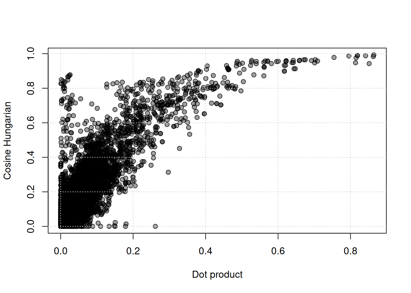
Summary
By translating between R and Python MS data structures, the SpectriPy package enables data analyses that combine functionalities from both programming language. In terms of (memory) efficiency, usage of SpectriPy’s MsBackendPy backend for Spectra objects has clear advantages over the repeated translation and copying of the MS data. See also section Section 5.1 for general comments.
Appendix
General comments
Be careful accessing Python attributes using
py$<attribute name>: base Python data types will be automatically converted to the equivalent R data type. For MS data, it might be better to get the attributes using thepy_get_attr()functions.Since MS data can be large, it is suggested the user converts MS data mostly manually, and only if/when needed, using
rspec_to_pyspec()andpyspec_to_rspec()- or, ideally, use aMsBackendPybackend.The
rspec_to_pyspec()andpyspec_to_rspec()functions copy the data while transferring. Thus, there will be eventually two (detached) copies of the same data in Python and R.The
MsBackendPybackend allows to directly interface MS data from Python. Data will be converted on-the-fly, so no additional copies of the data exist.Be aware that, since the
MsBackendPybackend does not contain any MS data but simply interfaces the MS data in Python, any changes to this data in Python affect also theSpectraobject using that backend.Be careful when re-assigning a
Spectraobject that uses aMsBackendPyto a new variable (e.g.b <- a, whereais such aSpectraobject). Both variables will point to the same Python variable and changing data/values in one of the variables will affect/change the data in the other variable (e.g. changing the MS level of all spectra inbusingb$msLevel <- 3will change the MS levels in the shared Python objects, hence,a$msLevelwill then also be3for all).
Session information
#' R session:

sessionInfo()
R version 4.6.0 (2026-04-24)
Platform: x86_64-pc-linux-gnu
Running under: Ubuntu 24.04.4 LTS
Matrix products: default
BLAS: /usr/lib/x86_64-linux-gnu/openblas-pthread/libblas.so.3
LAPACK: /usr/lib/x86_64-linux-gnu/openblas-pthread/libopenblasp-r0.3.26.so; LAPACK version 3.12.0
locale:
[1] LC_CTYPE=en_US.UTF-8 LC_NUMERIC=C
[3] LC_TIME=en_US.UTF-8 LC_COLLATE=en_US.UTF-8
[5] LC_MONETARY=en_US.UTF-8 LC_MESSAGES=en_US.UTF-8
[7] LC_PAPER=en_US.UTF-8 LC_NAME=C
[9] LC_ADDRESS=C LC_TELEPHONE=C
[11] LC_MEASUREMENT=en_US.UTF-8 LC_IDENTIFICATION=C
time zone: UTC
tzcode source: system (glibc)
attached base packages:
[1] stats4 stats graphics grDevices utils datasets methods
[8] base
other attached packages:
[1] MsBackendMgf_1.21.0 MsDataHub_1.13.0 SpectriPy_1.3.0
[4] reticulate_1.46.0 Spectra_1.23.0 BiocParallel_1.47.0
[7] S4Vectors_0.51.1 BiocGenerics_0.59.0 generics_0.1.4
loaded via a namespace (and not attached):
[1] KEGGREST_1.53.0 xfun_0.57 httr2_1.2.2
[4] Biobase_2.73.1 lattice_0.22-9 vctrs_0.7.3
[7] tools_4.6.0 curl_7.1.0 parallel_4.6.0
[10] tibble_3.3.1 AnnotationDbi_1.75.0 RSQLite_3.52.0
[13] cluster_2.1.8.2 blob_1.3.0 pkgconfig_2.0.3
[16] Matrix_1.7-5 data.table_1.18.4 dbplyr_2.5.2
[19] lifecycle_1.0.5 stringr_1.6.0 compiler_4.6.0
[22] Biostrings_2.81.1 BiocStyle_2.41.0 Seqinfo_1.3.0
[25] codetools_0.2-20 ncdf4_1.24 clue_0.3-68
[28] snakecase_0.11.1 htmltools_0.5.9 yaml_2.3.12
[31] crayon_1.5.3 pillar_1.11.1 MASS_7.3-65
[34] cachem_1.1.0 MetaboCoreUtils_1.21.1 ExperimentHub_3.3.0
[37] AnnotationHub_4.1.0 tidyselect_1.2.1 digest_0.6.39
[40] stringi_1.8.7 purrr_1.2.2 dplyr_1.2.1
[43] BiocVersion_3.24.0 fastmap_1.2.0 grid_4.6.0
[46] cli_3.6.6 magrittr_2.0.5 withr_3.0.2
[49] filelock_1.0.3 rappdirs_0.3.4 bit64_4.8.0
[52] XVector_0.53.0 httr_1.4.8 rmarkdown_2.31
[55] bit_4.6.0 otel_0.2.0 png_0.1-9
[58] memoise_2.0.1 evaluate_1.0.5 knitr_1.51
[61] IRanges_2.47.0 BiocFileCache_3.3.0 rlang_1.2.0
[64] Rcpp_1.1.1-1.1 glue_1.8.1 DBI_1.3.0
[67] mzR_2.47.0 BiocManager_1.30.27 jsonlite_2.0.0
[70] R6_2.6.1 fs_2.1.0 ProtGenerics_1.45.0
[73] MsCoreUtils_1.25.3