Introduction
This document shows how to access, use, and build annotation resources for untargeted metabolomics data. Reference spectral libraries are available from several sources, including:
-
GNPS: the Global Natural Products Social Molecular Networking (GNPS) is an open-access knowledge base for community-wide organization and sharing of raw, processed or identified MS/MS spectrometry data (Wang et al. 2016).
-
MassBank: MassBank is an open source mass spectral library for the identification of small chemical molecules of metabolomics, exposomics and environmental relevance (Neumann et al. 2025).
-
HMDB: the Human Metabolome Database (HMDB) is a freely available electronic database containing detailed information about small molecule metabolites found in the human body (Wishart et al. 2021).
-
MoNA: MassBank of North America (MoNA) is a metadata-centric, auto-curating repository for efficient storage and querying of mass spectral records.
Across resources, file formats, naming, and available annotations differ, so imports can be cumbersome. Packages exist for most formats, but harmonization remains challenging. Here we import public spectral libraries into data structures suitable for LC-MS/MS annotation, extract metadata, and outline future work toward harmonized formats such as mzSpecLib.
Accessing and using spectral libraries
Spectral libraries come in different formats. Packages from the RforMassSpectrometry initiative (MsBackendMgf, r Biocpkg("MsBackendMsp"), MsBackendMassbank, r Biocpkg("CompoundDb")) parse these formats into Spectra objects ready for R-based workflows. Below we load GNPS and MassBank libraries for LC-MS/MS annotation.
Using spectral libraries from GNPS
GNPS2 provides MS/MS spectral libraries, integrating data from sources such as MassBank and MoNA. Libraries are available as MGF, MSP, or JSON from the GNPS2 site and on Zenodo or Figshare with their own DOIs.
Here we download the GNPS2 drug library from Zenodo, a centralized collection of drug spectra with pharmacologic metadata (Zhao et al. 2025). We fetch all v4 resources (DOI: 10.5281/zenodo.17232042) to a temporary folder.
[1] "GNPS_Drug_Library_Metadata_Drug_Analogs_Updated_With_Source.csv"
[2] "GNPS_Drug_Library_Metadata_Drugs.csv"
[3] "GNPS_Drug_Library_Spectra_Drug_Analogs_Updated.mgf"
[4] "GNPS_Drug_Library_Spectra_Drugs_and_Metabolites.mgf"
The spectral libraries are available in MGF file format. Below we read the first 25 lines of the MGF file to inspect the available spectrum metadata fields.
mgf_fl <- file.path(pth, "GNPS_Drug_Library_Spectra_Drugs_and_Metabolites.mgf")
readLines(mgf_fl, n = 25)
 [1] "BEGIN IONS"
 [2] "PEPMASS=656.306"
 [3] "CHARGE=1"
 [4] "MSLEVEL=2"
 [5] "SOURCE_INSTRUMENT=LC-ESI-qTof"
 [6] "FILENAME=d10.mgf"
 [7] "SEQ=*..*"
 [8] "IONMODE=Positive"
 [9] "ORGANISM=GNPS-LIBRARY"
[10] "NAME=Rifamycin W M+H"
[11] "PI=Fenical-Jensen-Moore"
[12] "DATACOLLECTOR=Max"
[13] "SMILES=C[C@H]1/C=C/C=C(\\C(=O)NC2=CC(=O)C3=C(C(=C(C(=C3C2=O)O)C)O)C(=O)/C(=C/[C@@H]([C@@H]([C@H]([C@H]([C@@H]([C@@H]([C@@H]([C@H]1O)C)O)C)O)C)O)CO)/C)/C"
[14] "INCHI=InChI=1S/C35H45NO11/c1-14-9-8-10-15(2)35(47)36-22-12-23(38)24-25(32(44)20(7)33(45)26(24)34(22)46)28(40)16(3)11-21(13-37)31(43)19(6)30(42)18(5)29(41)17(4)27(14)39/h8-12,14,17-19,21,27,29-31,37,39,41-45H,13H2,1-7H3,(H,36,47)/b9-8+,15-10-,16-11+/t14-,17+,18+,19-,21+,27-,29+,30-,31+/m0/s1"
[15] "INCHIAUX=N/A"
[16] "PUBMED=N/A"
[17] "SUBMITUSER=mwang87"
[18] "LIBRARYQUALITY=1"
[19] "SPECTRUMID=CCMSLIB00000001635"
[20] "SCANS=1"
[21] "51.022472\t93.906502"
[22] "53.03849\t152.1483"
[23] "55.017834\t226.064896"
[24] "55.054722\t2069.459961"
[25] "56.056667\t98.109642"
The MGF format allows having additional fields to provide spectra metadata on top of mandatory fields such as PEPMASS (for precursor m/z) or CHARGE (for the precursor’s charge). MGF files can be imported into a Spectra object using the MsBackendMgf, which supports import of all metadata fields, renaming and mapping them to specific spectra variables. Below we define such a variable name mapping to map e.g. MSLEVEL to the spectra variable msLevel and NAME to spectrum_name.
We next import the MGF file into a Spectra object.
Start data import from 1 files ... done
We convert IONMODE from "Positive"/"Negative" to the standard polarity encoding (1/0).
drug_ms2$polarity[which(drug_ms2$IONMODE == "Positive")] <- 1L
drug_ms2$polarity[which(drug_ms2$IONMODE == "Negative")] <- 0L
Compound annotations are sparse in the imported library. Spectrum names hold the compound, adduct, and sometimes collision energy, but formatting is inconsistent:
drug_ms2$spectrum_name |>
    head()
[1] "Rifamycin W M+H"   "Rifamycin W M+Na"  "Dolastatin_10 M+H"
[4] "Rifamycin S M+Na"  "Rifamycin S M+H"   "phenazine M+H"
For these compounds, no charge or polarity information is provided, while for other compounds the adduct encoding follows more the standardized format.
drug_ms2$spectrum_name |>
    tail()
[1] "TRIMEBUTINE_metabolite_031 [[M+H]+]" "TRIMEDLURE [[M+H]+]"
[3] "TRIMEDLURE [[M+Na]+]"                "TRIMEDLURE [[M+K]+]"
[5] "TRIMEDLURE [[M+H-H2O]+]"             "Bictegravir [[M+H]+]"
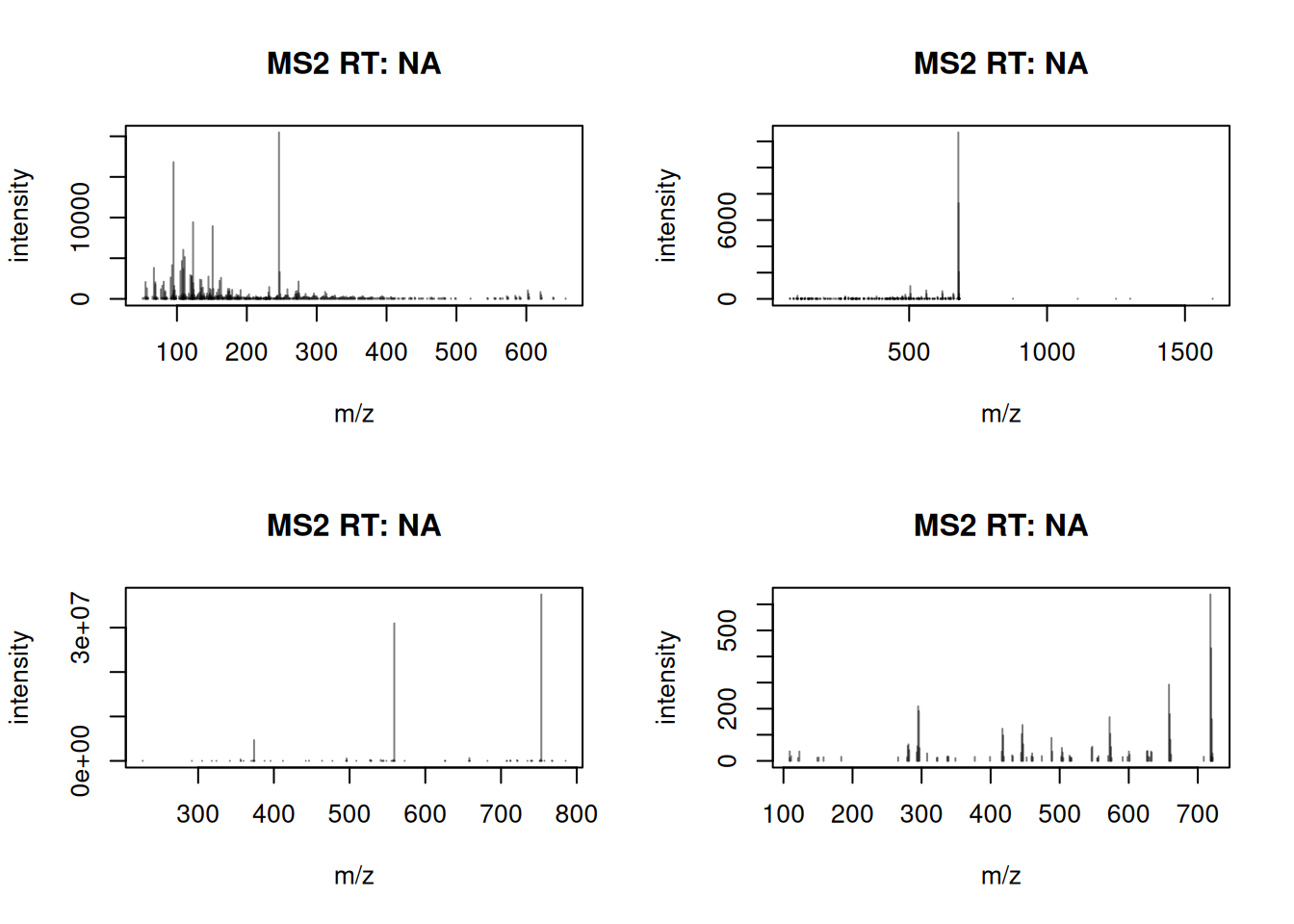
First examples how to extract and parse the adduct information are provided in the next section. For the present examples we simply use the data as provided. We first plot the first 4 reference spectra from the library.
Two things stand out: intensities are absolute, and a large number of low-abundance peaks are present likely reflecting instrument noise. We remove peaks below 1% of the maximum and scale intensities to sum to 1. This is one possible cleaning choice, not a standard.
drug_ms2 <- drug_ms2 |>
    #' remove peaks with intensity < 1% max intensity
    filterIntensity(intensity = function(x, ...) {
        x > max(x, na.rm = TRUE) / 100
    }) |>
    #' scale intensities to a total sum of 1
    scalePeaks()
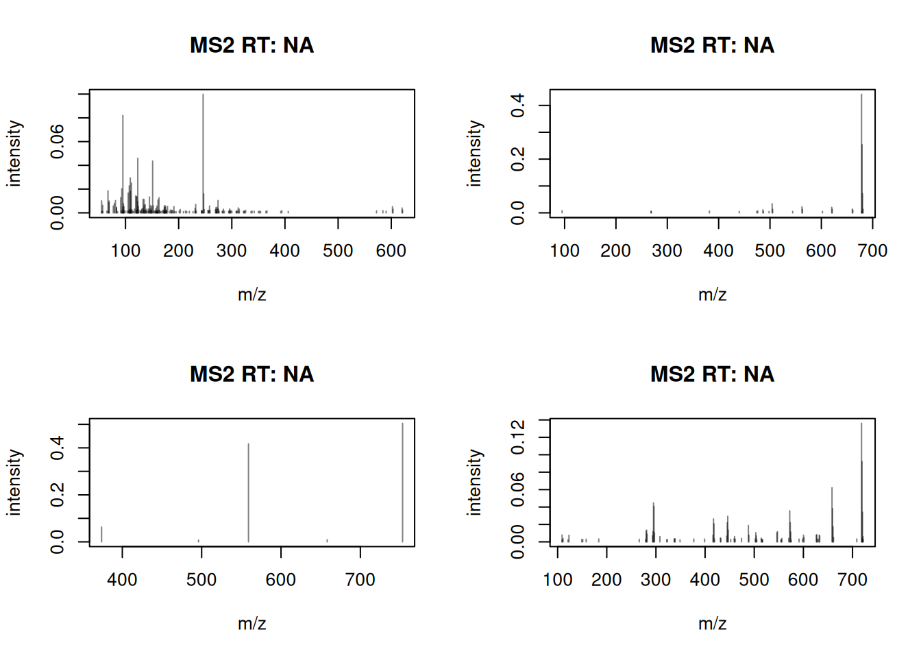
We plot the first 4 spectra again to evaluate the impact of this processing.
The number of fragment peaks per spectrum was thus reduced and intensities are now relative to the total intensity sum.
This Spectra object can now be used to match MS/MS spectra from the Complete end-to-end LC-MS/MS metabolomics data analysis workflow. We load the example Spectra object below.
#' load the MS2 spectra for significant features
fl <- system.file("extdata", "spectra_significant_fts.RData",
                  package = "Metabonaut")
load(fl) # ms2_ctr_fts
ms2_ctr_fts
MSn data (Spectra) with 315 spectra in a MsBackendMemory backend:
      msLevel     rtime scanIndex
    <integer> <numeric> <integer>
1           2   147.357      2043
2           2   148.587      2061
3           2   149.817      2079
4           2   152.297      2115
5           2   147.376      2041
...       ...       ...       ...
311         2   178.082      2481
312         2   179.322      2499
313         2   180.572      2517
314         2   181.822      2535
315         2   183.072      2553
 ... 39 more variables/columns.
Processing:
 Filter: select retention time [10..240] on MS level(s) 1 2 [Tue Mar 18 11:56:42 2025]
 Filter: select MS level(s) 2 [Tue Mar 18 11:56:50 2025]
 Remove peaks based on their intensities and a user-provided function in spectra of MS level(s) 2. [Tue Mar 18 11:56:50 2025]
 ...19 more processings. Use 'processingLog' to list all.
This Spectra object contains MS/MS spectra for features with significant abundance differences. We match them against the GNPS2 drug library with MetaboAnnotation.
And, not unexpectedly, most fragment spectra match to reference spectra for caffeine.
res$target_spectrum_name |> unique()
 [1] "caffeine M+H"
 [2] "Methazolastone M+H"
 [3] "1,3,7-trimethyl-3,7-dihydro-1H-purine-2,6-dione [M+H]+"
 [4] "Massbank:BML00705 Caffeine [M+H]+"
 [5] "Massbank:EA030301 Caffeine|1,3,7-trimethyl-3,7-dihydro-1H-purine-2,6-dione|1,3,7-trimethylpurine-2,6-dione [M+H]+"
 [6] "Massbank:EA030311 Caffeine|1,3,7-trimethyl-3,7-dihydro-1H-purine-2,6-dione|1,3,7-trimethylpurine-2,6-dione [M+H]+"
 [7] "Massbank:EA030312 Caffeine|1,3,7-trimethyl-3,7-dihydro-1H-purine-2,6-dione|1,3,7-trimethylpurine-2,6-dione [M+H]+"
 [8] "Massbank:EA030314 Caffeine|1,3,7-trimethyl-3,7-dihydro-1H-purine-2,6-dione|1,3,7-trimethylpurine-2,6-dione [M+H]+"
 [9] "Massbank:FIO00570 Caffeine [M+H]+"
[10] "Massbank:MT000087 Caffeine [M+H]+"
[11] "Massbank:UF408902 Caffeine|1,3,7-trimethyl-3,7-dihydro-1H-purine-2,6-dione|1,3,7-trimethylpurine-2,6-dione [M+H]+"
[12] "Massbank:UF408903 Caffeine|1,3,7-trimethyl-3,7-dihydro-1H-purine-2,6-dione|1,3,7-trimethylpurine-2,6-dione [M+H]+"
[13] "Massbank:UF408904 Caffeine|1,3,7-trimethyl-3,7-dihydro-1H-purine-2,6-dione|1,3,7-trimethylpurine-2,6-dione [M+H]+"
[14] "Massbank:KW107904 caffeine M+H"
[15] "Massbank:KW107901 caffeine M+H"
[16] "Massbank:LU119904 Caffeine|1,3,7-trimethylpurine-2,6-dione M+H"
[17] "MassbankEU:UA005001 Caffeine|1,3,7-trimethylpurine-2,6-dione [M+H]+"
[18] "Caffeine - 30.0 eV M+H"
[19] "CAFFEINE - 60.0 eV M+H"
[20] "Massbank:EA030306 Caffeine|1,3,7-trimethyl-3,7-dihydro-1H-purine-2,6-dione|1,3,7-trimethylpurine-2,6-dione [M+H]+"
[21] "CAFFEINE M+H"
[22] "CAFFEINE - 70.0 eV M+H"
[23] "Caffeine [M+H]+"
[24] "Massbank:EA030305 Caffeine|1,3,7-trimethyl-3,7-dihydro-1H-purine-2,6-dione|1,3,7-trimethylpurine-2,6-dione [M+H]+"
[25] "Massbank:EA030307 Caffeine|1,3,7-trimethyl-3,7-dihydro-1H-purine-2,6-dione|1,3,7-trimethylpurine-2,6-dione [M+H]+"
[26] "Massbank:EA030313 Caffeine|1,3,7-trimethyl-3,7-dihydro-1H-purine-2,6-dione|1,3,7-trimethylpurine-2,6-dione [M+H]+"
[27] "Massbank:LU119905 Caffeine|1,3,7-trimethylpurine-2,6-dione M+H"
To summarize, through packages such as MsBackendMgf, r Biocpkg("MsBackendMsp") it is easily possible to integrate public (or in-house) spectral reference libraries in MGF or MSP file format into R-based annotation workflows.
Importing and cleaning GNPS MGF files using Python’s matchms library
Alternatively, it is possible to import and clean the GNPS MGF file in Python with matchms and access it in R through MsBackendPy from the r Biocpkg("SpectriPy") package (Graeve et al. 2025).
#' load the required SpectriPy package; this will also install
#' eventually required Python libraries and dependencies
library(SpectriPy)
Loading required package: reticulate
We next import the MGF file in Python using the matchms library (Huber et al. 2020).
import matchms
from matchms.importing import load_from_mgf

#' import the fragment spectra from the MGF file
s_py = list(load_from_mgf(r.mgf_fl))
Next we clean and harmonize metadata with matchms filters. See the matchms.filtering documentation or (Jonge et al. 2024) for options.
from matchms.filtering import default_filters, clean_adduct

#' apply filters to clean the spectra metadata
s_py_clean = []
for s in s_py:
    s = default_filters(s)
    s = clean_adduct(s)
    s_py_clean.append(s)

#' delete the unfiltered data
del s_py
To access the cleaned spectra data we create next a Spectra object using SpectriPy’s MsBackendPy backend.
 [1] "msLevel"                 "rtime"
 [3] "acquisitionNum"          "scanIndex"
 [5] "dataStorage"             "dataOrigin"
 [7] "centroided"              "smoothed"
 [9] "polarity"                "precScanNum"
[11] "precursorMz"             "precursorIntensity"
[13] "precursorCharge"         "collisionEnergy"
[15] "isolationWindowLowerMz"  "isolationWindowTargetMz"
[17] "isolationWindowUpperMz"  "adduct"
[19] "compound_name"           "confidence"
[21] "data_collector"          "file_name"
[23] "inchi"                   "instrument_type"
[25] "ionmode"                 "organism_name"
[27] "peptide_sequence"        "principal_investigator"
[29] "scans"                   "smiles"
[31] "spectrum_id"             "submit_user"
The adduct information was now harmonized by the filtering workflow in Python:
#' get the unique adduct types
table(s_py$adduct)
         [2M-2H+Na]-              [2M-H]-           [2M-H+Na]-
                 139                  293                    1
          [2M+FA-H]-              [2M+H]+           [2M+K-2H]-
                   1                  253                    1
             [2M+K]+          [2M+Na-2H]-             [2M+Na]+
                  10                    1                  120
           [2M+NH4]+              [3M-H]-              [3M+H]+
                   4                    2                    1
            [3M+Na]+            [3M+NH4]+        [M-2(H2O)+H]+
                   1                    1                    1
             [M-2H]-             [M-2H]2-          [M-2H2O+H]+
                   1                   41                   84
         [M-3H2O+H]+               [M-e]-               [M-H]-
                   2                   12                12731
          [M-H+H2O]-         [M-H+HCOOH]-            [M-H+Na]+
                   1                    2                    6
          [M-H2O-H]-             [M-H2O]+           [M-H2O+H]+
                   1                    1                  531
                [M]+             [M+2H]2+           [M+2Na-H]+
                  88                  275                   55
           [M+2Na]2+             [M+3H]3+           [M+ACN+H]+
                   2                    1                    3
              [M+C]-             [M+Ca]2+          [M+CH3COO]-
                   1                    1                   20
[M+CH3COO]-/[M-CH3]-         [M+CH3OH+H]+              [M+Cl]-
                   7                    1                  162
           [M+FA-H]-          [M+H-3H2O]+         [M+H-C2H5N]+
                  11                    5                    1
         [M+H-C4H6]+       [M+H-C5H12N2]+       [M+H-C5H9NO4]+
                   1                    5                    1
          [M+H-H20]+           [M+H-NH3]+               [M+H]+
                   1                    4                68444
           [M+HCOO]-               [M+K]+              [M+Li]+
                  88                  465                    2
          [M+Na-2H]-              [M+Na]+             [M+NH4]+
                   2                13947                  551
The s_py Spectra object is ready for R workflows. Data stay in Python and is translated on demand; switch to MsBackendMemory to copy it to R if needed.
Using MassBank data
MassBank was one of the first open-source and open access cross-vendor mass spectral libraries (Neumann et al. 2025). All content, which is validated using automatic pipelines, is under version control and versioned releases are pushed to an independent data repository. The easiest way to use MassBank annotations in R is to get the respective database from Bioconductor’s AnnotationHub. This is also described in more detail in the MS1-based annotation section in the main end-to-end workflow. Below we first load the respective library and the list of available annotations from AnnotationHub.
AnnotationHub can then be queried for MassBank records:
        id                           description
1 AH107048   MassBank CompDb for release 2021.03
2 AH107049   MassBank CompDb for release 2022.06
3 AH111334 MassBank CompDb for release 2022.12.1
4 AH116164   MassBank CompDb for release 2023.06
5 AH116165   MassBank CompDb for release 2023.09
6 AH116166   MassBank CompDb for release 2023.11
7 AH119518   MassBank CompDb for release 2024.06
8 AH119519   MassBank CompDb for release 2024.11
And a specific MassBank release can then be loaded using the respective AnnotationHub identifier. Below we load data from MassBank release 2023.11.
class: CompDb
 data source: MassBank
 version: 2023.11
 organism: NA
 compound count: 117732
 MS/MS spectra count: 117732
The result is returned as a CompDb object from the CompoundDb package which can be directly used with the annotation functions from the r Biocpkg("MetaboAnnotation") package. While this approach is convenient and fast, not all MassBank releases are available through AnnotationHub.
Alternatively, download MassBank data from the MassBank GitHub page or Zenodo. DOI 10.5281/zenodo.3378723 points to the latest release. Here we fetch release 2025.10 via DOI 10.5281/zenodo.17432277:
[1] "MassBank-data-2025.10.zip"
The archive contains several thousands of .txt files in MassBank format, one for each spectrum. We next unzip the archive to the same temporary folder and get the listing of all data files.
#' unzip the archive
unzip(file.path(pth, dir(pth)[1L]), exdir = pth)

#' get the file listing
dr <- dir(pth, pattern = "MassBank-MassBank", full.names = TRUE)
fls <- dir(dr, recursive = TRUE, pattern = "txt$", full.names = TRUE)
length(fls)
Each file holds one spectrum with compound, instrument, and provider metadata in MassBank format. We import the full release with MsBackendMassbank() into a Spectra object.
MSn data (Spectra) with 134440 spectra in a MsBackendMassbank backend:
         msLevel     rtime scanIndex
       <integer> <numeric> <integer>
1              2      3.44         1
2              2      3.44         1
3              2      3.44         1
4              2      3.44         1
5              2      3.44         1
...          ...       ...       ...
134436         2     685.2         1
134437         2     685.2         1
134438         2     685.2         1
134439         2     685.2         1
134440         2     685.2         1
 ... 28 more variables/columns.
Metadata and annotations of the compound are available as additional spectra variables, such as "name", "smiles", "formula", "inchi" etc. The full list of available spectra metadata is:
 [1] "msLevel"                 "rtime"
 [3] "acquisitionNum"          "scanIndex"
 [5] "dataStorage"             "dataOrigin"
 [7] "centroided"              "smoothed"
 [9] "polarity"                "precScanNum"
[11] "precursorMz"             "precursorIntensity"
[13] "precursorCharge"         "collisionEnergy"
[15] "isolationWindowLowerMz"  "isolationWindowTargetMz"
[17] "isolationWindowUpperMz"  "acquistionNum"
[19] "accession"               "name"
[21] "smiles"                  "exactmass"
[23] "formula"                 "inchi"
[25] "cas"                     "inchikey"
[27] "adduct"                  "splash"
[29] "title"
The metaBlocks parameter can be used to enable import of extra metadata. MassBank metadata are generally more standardized and include more compound information (e.g., formula, exact mass). We now match the end-to-end vignette spectra against MassBank 2025.10 with matchSpectra().
The experimental spectra match against spectra of compounds with the following unique InChI:
[1] "InChI=1S/C9H6O3/c10-7-5-9(11)12-8-4-2-1-3-6(7)8/h1-5,10H"
[2] "InChI=1S/C7H13N5O/c1-3-8-5-10-6(9-4-2)12-7(13)11-5/h3-4H2,1-2H3,(H3,8,9,10,11,12,13)"
[3] "InChI=1S/C8H10N4O2/c1-10-4-9-6-5(10)7(13)12(3)8(14)11(6)2/h4H,1-3H3"
The names (including aliases) of the compounds are:
 [1] "4-Hydroxycoumarin"
 [2] "4-hydroxychromen-2-one"
 [3] "Simazine-2-hydroxy"
 [4] "4,6-bis(ethylamino)-1H-1,3,5-triazin-2-one"
 [5] "2-Hydroxysimazine"
 [6] "2,6-bis(ethylamino)-1H-1,3,5-triazin-4-one"
 [7] "Caffeine"
 [8] "1,3,7-trimethyl-3,7-dihydro-1H-purine-2,6-dione"
 [9] "1,3,7-trimethylpurine-2,6-dione"
[10] "caffeine"
[11] "CAFFEINE"
[12] "1,3,7-Trimethylpurine-2,6-dione"
Creating or expanding annotation resources
Public MGF/MSP libraries can be imported into Spectra and exported again. Alternatively, annotations can be stored in SQL databases via the r Biocpkg("CompoundDb") package, which defines a simple database schema for small compounds and MS data. Here we build a database from the GNPS2 drug library; see the vignette Creating CompoundDb annotation resources for more examples.
Note
The CompDb database layout defines 3 main database tables, one for compound annotations, one for spectra metadata and one to store the actual mass (or fragment) peaks. These tables are linked with each other through specific identifier columns (primary/foreign keys): each table has its own ID column with unique identifiers for each row. To link the MS spectra tables with the compound annotation table, the table with the MS spectra metadata contains in addition a column with the identifiers of the compound the specific fragment spectrum is associated with. An additional table metadata allows to define metadata information for the full annotation resource, such as a version, origin, DOI, etc.
We first define a data.frame with compound annotations for the GNPS2 drug library. The MGF metadata mainly describe spectrum generation, with compound details mostly in the spectrum name and INCHI. Spectrum names often mix in collision energy and ion information and are not standardized:
library(CompoundDb)

#' extract potential compound relevant information
cmps <- spectraData(drug_ms2, c("ORGANISM", "spectrum_name", "inchi",
                                "smiles", "exactmass")) |>
    as.data.frame()

#' inspect values for the spectrum name
cmps$spectrum_name |> head()
[1] "Rifamycin W M+H"   "Rifamycin W M+Na"  "Dolastatin_10 M+H"
[4] "Rifamycin S M+Na"  "Rifamycin S M+H"   "phenazine M+H"
cmps$spectrum_name |> tail()
[1] "TRIMEBUTINE_metabolite_031 [[M+H]+]" "TRIMEDLURE [[M+H]+]"
[3] "TRIMEDLURE [[M+Na]+]"                "TRIMEDLURE [[M+K]+]"
[5] "TRIMEDLURE [[M+H-H2O]+]"             "Bictegravir [[M+H]+]"
cmps$spectrum_name[1000:1006]
[1] "ISOLEUCINE - 20.0 eV M+H" "ISOLEUCINE - 30.0 eV M+H"
[3] "ISOLEUCINE - 40.0 eV M+H" "ISOLEUCINE - 50.0 eV M+H"
[5] "ISOLEUCINE - 60.0 eV M+H" "ISOLEUCINE - 70.0 eV M+H"
[7] "GLUTAMATE - 20.0 eV M+H"
To define the names for the compounds we first parse (and then strip) the adduct information from the spectrum name. The pattern defined below finds all sub-strings that start with a white space, followed by no, one or two "[", an "M" (or "2M" etc) with a "+" or a "-" followed by any character until the end of the string. This patter should allow to find all adduct definitions, even if they don’t follow the standard nomenclature.
sname <- cmps$spectrum_name

#' define the pattern for adduct definitions
paddct <- "\\s(\\[{0,2}\\d?M)(\\]|\\+|-|$).*$"

#' extract the adduct definition from the spectrum names
library(stringr)
addct <- str_extract(sname, paddct) |>
    str_trim()
head(unique(addct))
[1] "M+H" "M+Na" "M+2H" NA "M-H" "M+H-H20"
[1] "M+C"          "[[M+H]+]"     "[[M+K]+]"     "[[M+H-H2O]+]" "[[M+Na]+]"
[6] "[[M]+]"
Ideally we would standardize adducts (e.g., convert "M+H" or "[[M+H]+]" to "[M+H]+"), but here we keep the provided values and store them as a new adduct variable.
#' create a new spectra variable with adduct information
drug_ms2$adduct <- addct
We strip adducts from the spectrum names, drop trailing " Unknown", and remove extra quotes.
#' remove any adduct definitions from the compound name
cname <- sub(paddct, "", sname) |>
    sub(pattern = "\\sUnknown$", replacement = "") |>
    gsub(pattern = "\"", replacement = "")
For some spectra also the collision energy was included in the name. Some examples are:
cname[c(844, 845, 8845, 8846, 69316, 9762, 9763)]
[1] "TYRAMINE - 20.0 eV"                "TYRAMINE - 30.0 eV"
[3] "Benzylpenicillin_40eV"             "Benzylpenicillin_50eV"
[5] "Daidzein - 50eV"                   "tryptophan CollisionEnergy:205060"
[7] "tryptophan CollisionEnergy:102040"
We define a pattern to capture these collision energy definitions and strip it from the compound names.
pce1 <- "(_|\\s-\\s|\\s)(\\d*.*)eV$"
pce2 <- " CollisionEnergy:\\d+$"
cname <- sub(pattern = pce1, replacement = "", cname) |>
    sub(pattern = pce2, replacement = "")
Some spectrum names also include the original database ID:
cname[c(36925, 56836, 57333, 68442)]
[1] "Massbank:BML00001 Cytisine"
[2] "MassbankEU:ET010001 CLC_301.1468_14.3|Chlorcyclizine|1-[(4-chlorophenyl)-phenylmethyl]-4-methylpiperazine"
[3] "MoNA:2504 Ceftiofur"
[4] "HMDB:HMDB00145-218 Estrone"
Ideally we would split these IDs into separate columns; here we keep them in the compound name, rename ORGANISM to data_origin, and ensure exactmass is numeric.
#' add compound names to the data.frame
cmps$name <- cname
#' remove unneded columns
cmps$spectrum_name <- NULL
#' rename "ORGANISM" column name to "data_origin"
colnames(cmps) <- sub("ORGANISM", "data_origin", colnames(cmps))
#' ensure column exactmass is of type numeric
cmps$exactmass <- as.numeric(cmps$exactmass)
We clean smiles and inchi by trimming whitespace, removing "N/A", and dropping extra quotes.
#' excess "
cmps$inchi <- gsub("\"", "", cmps$inchi)
cmps$smiles <- gsub("\"", "", cmps$smiles)
#' white spaces
cmps$inchi <- str_trim(cmps$inchi)
cmps$smiles <- str_trim(cmps$smiles)
#' NA encodings
cmps$inchi[cmps$inchi == ""] <- NA_character_
cmps$inchi <- sub("^N/A", NA_character_, cmps$inchi)
cmps$smiles[cmps$smiles == ""] <- NA_character_
cmps$smiles <- sub("^N/A", NA_character_, cmps$smiles)
Finally, we add remaining required columns "inchikey", "formula" and "synonyms". No related information was provided in the input MGF and we thus fill these with NA.
#' add missing columns and initialize with NA
cmps$inchikey <- NA_character_
cmps$formula <- NA_character_
cmps$synonyms <- NA_character_
Next we define spectra metadata. Suggested columns include polarity (0/1/NA), collision_energy, instrument, instrument_type, and precursor_mz with CompoundDb accepting also optional additional columns. We extract these from the GNPS2 Spectra object into a data.frame.
#' extract the spectra information and data
spctra <- spectraData(drug_ms2,
                      c("spectrum_name",
                        "polarity",
                        "collisionEnergy",
                        "FILENAME",
                        "PI",
                        "DATACOLLECTOR",
                        "PUBMED",
                        "LIBRARYQUALITY",
                        "SPECTRUMID",
                        "SOURCE_INSTRUMENT",
                        "precursorMz",
                        "mz",
                        "intensity")
                      ) |>
    as.data.frame()
We rename SOURCE_INSTRUMENT to instrument_type, add an empty instrument column, and replace "N/A" with NA.
#' add instrument information
colnames(spctra) <- sub("SOURCE_INSTRUMENT", "instrument_type",
                        colnames(spctra))
spctra$instrument <- NA_character_
#' fix missing values
spctra$PI <- sub("^N/A", NA_character_, spctra$PI)
spctra$DATACOLLECTOR <- sub("^N/A", NA_character_, spctra$DATACOLLECTOR)
spctra$PUBMED <- sub("^N/A", NA_character_, spctra$PUBMED)
We standardize column names to match Spectra/CompoundDb conventions.
To allow linking spectra to compounds (i.e., rows in the cmps with rows in the spctra data frames) we add unique IDs for each table.
Ideally compounds would be unique and spectra could map many-to-one. Here each compound row corresponds to one spectrum, so we add compound_id directly to spctra.
#' define the relationship between spectra and compounds
spctra$compound_id <- cmps$compound_id
Finally we define database metadata (origin, version, DOI) for reproducibility.
#' define metadata for the annotation resource
metad <- make_metadata(source = "GNPS",
                       url = "https://doi.org/10.5281/zenodo.17232042",
                       source_version = "v4",
                       source_date = "2025-09-30",
                       organism = NA_character_)
Now, with all tables and relevant information available, we can create the SQLite-based annotation resource using the createCompDb() function
#' create an annotation database in CompDb format
db_file <- createCompDb(cmps,
                        metadata = metad,
                        msms_spectra = spctra,
                        dbFile = "GNPS-drug-library.v4.sqlite")
All tables are stored in the SQLite file ./GNPS-drug-library.v4.sqlite, usable with any SQLite client. Below we connect with RSQLite and list tables.
library(RSQLite)
#' connect to the database
con <- dbConnect(SQLite(), db_file)
#' list the available tables
dbListTables(con)
[1] "metadata"           "ms_compound"        "msms_spectrum"
[4] "msms_spectrum_peak" "synonym"
We could also use SQL queries to retrieve data from this database. For example we extract below the first 10 entries of the database table with the mass peak data.
#' get first 10 rows of the peak data table
dbGetQuery(con, "select * from msms_spectrum_peak limit 10")
   spectrum_id       mz   intensity peak_id
1            1 55.01783 0.001102225       1
2            1 55.05472 0.010090073       2
3            1 57.03398 0.006352579       3
4            1 57.06980 0.001213007       4
5            1 65.03873 0.001344491       5
6            1 67.05451 0.018575616       6
7            1 68.05765 0.001046733       7
8            1 69.03366 0.008645037       8
9            1 69.06998 0.009978069       9
10           1 77.03866 0.005749947      10
#' disconnect from the database
dbDisconnect(con)
For direct use, we load the database as a CompDb annotation resource:
class: CompDb
 data source: GNPS
 version: v4
 organism: NA
 compound count: 105856
 MS/MS spectra count: 105856
This simplifies access via CompoundDb functions such as compounds(), filter(), and metadata().
#' get the resource's metadata
metadata(cdb)
                name                                   value
1             source                                    GNPS
2                url https://doi.org/10.5281/zenodo.17232042
3     source_version                                      v4
4        source_date                              2025-09-30
5           organism                                    <NA>
6   db_creation_date                Tue Mar 17 16:21:08 2026
7 supporting_package                              CompoundDb
8  supporting_object                                  CompDb
For MS2 workflows, interface with the CompDb via a Spectra object.
#' access the annotation resource as a `Spectra` object
sps_cdb <- Spectra(cdb)
sps_cdb
MSn data (Spectra) with 105856 spectra in a MsBackendCompDb backend:
         msLevel precursorMz  polarity
       <integer>   <numeric> <integer>
1             NA     656.306         1
2             NA     678.290         1
3             NA     785.230         1
4             NA     718.286         1
5             NA     696.304         1
...          ...         ...       ...
105852        NA     233.131         1
105853        NA     255.113         1
105854        NA     271.087         1
105855        NA     215.120         1
105856        NA     450.127         1
 ... 39 more variables/columns.
 Use  'spectraVariables' to list all of them.
 data source: GNPS
 version: v4
 organism: NA
This Spectra object can then be used for annotation workflows as described in the previous section or the MS2-based annotation section of the main Complete end-to-end LC-MS/MS Metabolomic Data analysis workflow.
The Spectra ecosystem loads MS data from many formats, enabling integration of diverse libraries into R workflows.
MGF and MSP are common exchange formats but repeat compound annotations for every spectrum. Loading them requires reading all data, which can be slow and memory-heavy for large libraries.
For example, the memory usage for the GNPS drug library imported from the MGF file is
This file is manageable; the full GNPS library might exceed the available memory of a standard computer.
In contrast, the memory size for the Spectra object of the CompDb annotation database created from the GNPS2 drug library is only:
The sps_cdb Spectra object keeps only spectrum IDs in memory and fetches other data on demand, keeping memory low.
Another advantage of CompDb resources over MGF/MSP-based file formats is the possibility to assign metadata to the resource:
                name                                   value
1             source                                    GNPS
2                url https://doi.org/10.5281/zenodo.17232042
3     source_version                                      v4
4        source_date                              2025-09-30
5           organism                                    <NA>
6   db_creation_date                Tue Mar 17 16:21:08 2026
7 supporting_package                              CompoundDb
8  supporting_object                                  CompDb
However, creating a CompDb requires an upfront cleanup and conversion to store data in SQLite. Once built, the resource is self-contained and shareable.
The CompDb format also supports adding new compounds or spectra, enabling extension of in-house libraries (see the CompoundDb vignette mentioned above).
Currently the format is only supported directly in R, though any SQLite client can read the database.
Summary
Importing public reference libraries is straightforward. The challenge is harmonizing metadata and annotations across sources. Interpretation benefits from cleaned, standardized information. Efforts such as (Jonge et al. 2024) help, but broader standardization of data and naming conventions is still needed.
Outlook
- Support for the newly defined mzSpecLib file format will be added to the RforMassSpectrometry package ecosystem.
- Access to public libraries will be simplified, e.g. by making them available through AnnotationHub.
R version 4.5.2 (2025-10-31)
Platform: x86_64-pc-linux-gnu
Running under: Ubuntu 24.04.3 LTS

Matrix products: default
BLAS:   /usr/lib/x86_64-linux-gnu/openblas-pthread/libblas.so.3
LAPACK: /usr/lib/x86_64-linux-gnu/openblas-pthread/libopenblasp-r0.3.26.so;  LAPACK version 3.12.0

locale:
 [1] LC_CTYPE=en_US.UTF-8       LC_NUMERIC=C
 [3] LC_TIME=en_US.UTF-8        LC_COLLATE=en_US.UTF-8
 [5] LC_MONETARY=en_US.UTF-8    LC_MESSAGES=en_US.UTF-8
 [7] LC_PAPER=en_US.UTF-8       LC_NAME=C
 [9] LC_ADDRESS=C               LC_TELEPHONE=C
[11] LC_MEASUREMENT=en_US.UTF-8 LC_IDENTIFICATION=C

time zone: Etc/UTC
tzcode source: system (glibc)

attached base packages:
[1] stats4    stats     graphics  grDevices utils     datasets  methods
[8] base

other attached packages:
 [1] RSQLite_2.4.6            stringr_1.6.0            MsBackendMassbank_1.18.2
 [4] CompoundDb_1.14.2        AnnotationFilter_1.34.0  AnnotationHub_4.0.0
 [7] BiocFileCache_3.0.0      dbplyr_2.5.2             SpectriPy_1.0.1
[10] reticulate_1.45.0        MetaboAnnotation_1.14.0  MsBackendMgf_1.18.0
[13] zen4R_0.10.4             Spectra_1.20.1           BiocParallel_1.44.0
[16] S4Vectors_0.48.0         BiocGenerics_0.56.0      generics_0.1.4
[19] BiocStyle_2.38.0         quarto_1.5.1.9002        knitr_1.51

loaded via a namespace (and not attached):
  [1] DBI_1.3.0                   bitops_1.0-9
  [3] httr2_1.2.2                 gridExtra_2.3
  [5] rlang_1.1.7                 magrittr_2.0.4
  [7] clue_0.3-67                 otel_0.2.0
  [9] matrixStats_1.5.0           compiler_4.5.2
 [11] png_0.1-9                   vctrs_0.7.1
 [13] reshape2_1.4.5              ProtGenerics_1.42.0
 [15] crayon_1.5.3                pkgconfig_2.0.3
 [17] MetaboCoreUtils_1.18.1      fastmap_1.2.0
 [19] XVector_0.50.0              utf8_1.2.6
 [21] rmarkdown_2.30              ps_1.9.1
 [23] purrr_1.2.1                 bit_4.6.0
 [25] xfun_0.56                   MultiAssayExperiment_1.36.1
 [27] cachem_1.1.0                ChemmineR_3.62.0
 [29] jsonlite_2.0.0              blob_1.3.0
 [31] later_1.4.8                 DelayedArray_0.36.0
 [33] parallel_4.5.2              cluster_2.1.8.2
 [35] R6_2.6.1                    stringi_1.8.7
 [37] RColorBrewer_1.1-3          GenomicRanges_1.62.1
 [39] Rcpp_1.1.1                  Seqinfo_1.0.0
 [41] SummarizedExperiment_1.40.0 base64enc_0.1-6
 [43] IRanges_2.44.0              BiocBaseUtils_1.12.0
 [45] Matrix_1.7-4                igraph_2.2.2
 [47] tidyselect_1.2.1            rstudioapi_0.18.0
 [49] abind_1.4-8                 yaml_2.3.12
 [51] codetools_0.2-20            curl_7.0.0
 [53] processx_3.8.6              lattice_0.22-9
 [55] tibble_3.3.1                plyr_1.8.9
 [57] withr_3.0.2                 KEGGREST_1.50.0
 [59] Biobase_2.70.0              S7_0.2.1
 [61] evaluate_1.0.5              xml2_1.5.2
 [63] Biostrings_2.78.0           filelock_1.0.3
 [65] pillar_1.11.1               BiocManager_1.30.27
 [67] MatrixGenerics_1.22.0       DT_0.34.0
 [69] rprojroot_2.1.1             RCurl_1.98-1.17
 [71] BiocVersion_3.22.0          ggplot2_4.0.2
 [73] scales_1.4.0                glue_1.8.0
 [75] lazyeval_0.2.2              tools_4.5.2
 [77] data.table_1.18.2.1         QFeatures_1.20.0
 [79] fs_1.6.7                    XML_3.99-0.22
 [81] grid_4.5.2                  tidyr_1.3.2
 [83] AnnotationDbi_1.72.0        MsCoreUtils_1.22.1
 [85] cli_3.6.5                   rappdirs_0.3.4
 [87] rsvg_2.7.0                  S4Arrays_1.10.1
 [89] keyring_1.4.1.9000          dplyr_1.2.0
 [91] gtable_0.3.6                digest_0.6.39
 [93] SparseArray_1.10.9          rjson_0.2.23
 [95] htmlwidgets_1.6.4           farver_2.1.2
 [97] memoise_2.0.1               htmltools_0.5.9
 [99] lifecycle_1.0.5             here_1.0.2
[101] httr_1.4.8                  bit64_4.6.0-1
[103] MASS_7.3-65
References
Graeve, Marilyn De, Wout Bittremieux, Thomas Naake, Carolin Huber, Matthias Anagho-Mattanovich, Nils Hoffmann, Pierre Marchal, et al. 2025.
“SpectriPy: Enhancing Cross-Language Mass Spectrometry Data Analysis with R and Python.” Journal of Open Source Software 10 (109): 8070.
https://doi.org/10.21105/joss.08070.
Huber, Florian, Stefan Verhoeven, Christiaan Meijer, Hanno Spreeuw, Efraín Manuel Villanueva Castilla, Cunliang Geng, Justin J. j van der Hooft, et al. 2020.
“Matchms - Processing and Similarity Evaluation of Mass Spectrometry Data.” Journal of Open Source Software 5 (52): 2411.
https://doi.org/10.21105/joss.02411.
Jonge, Niek F. de, Helge Hecht, Michael Strobel, Mingxun Wang, Justin J. J. van der Hooft, and Florian Huber. 2024.
“Reproducible MS/MS Library Cleaning Pipeline in Matchms.” Journal of Cheminformatics 16 (1): 88.
https://doi.org/10.1186/s13321-024-00878-1.
Neumann, Steffen, René Meier, Michael Wenk, Anjana Elapavalore, Takaaki Nishioka, Tobias Schulze, Michael Stravs, Hiroshi Tsugawa, Fumio Matsuda, and Emma L. Schymanski. 2025.
“MassBank: An Open and FAIR Mass Spectral Data Resource.” Nucleic Acids Research, November, gkaf1193.
https://doi.org/10.1093/nar/gkaf1193.
Wang, Mingxun, Jeremy J. Carver, Vanessa V. Phelan, Laura M. Sanchez, Neha Garg, Yao Peng, Don Duy Nguyen, et al. 2016.
“Sharing and Community Curation of Mass Spectrometry Data with Global Natural Products Social Molecular Networking.” Nature Biotechnology 34 (8): 828–37.
https://doi.org/10.1038/nbt.3597.
Wishart, David S, AnChi Guo, Eponine Oler, Fei Wang, Afia Anjum, Harrison Peters, Raynard Dizon, et al. 2021.
“HMDB 5.0: The Human Metabolome Database for 2022.” Nucleic Acids Research 50 (D1): D622–31.
https://doi.org/10.1093/nar/gkab1062.
Zhao, Haoqi Nina, Kine Eide Kvitne, Corinna Brungs, Siddharth Mohan, Vincent Charron-Lamoureux, Wout Bittremieux, Runbang Tang, et al. 2025.
“A Resource to Empirically Establish Drug Exposure Records Directly from Untargeted Metabolomics Data.” Nature Communications 16 (1): 10600.
https://doi.org/10.1038/s41467-025-65993-5.