Chapter 4 Identification data
Peptide identification is performed using third-party software - there
is no package to run these searches directly in R. When using command
line search engines it possible to hard-code or automatically generate
the search command lines and run them from R using a system()
call. This allows to generate these reproducibly (especially useful if
many command lines need to be run) and to keep a record in the R
script of the exact command.
The example below illustrates this for 3 mzML files to be searched
using MSGFplus:
## [1] "file_1.mzML" "file_2.mzML" "file_3.mzML"## [1] "file_1.mzid" "file_2.mzid" "file_3.mzid"paste0("java -jar /path/to/MSGFPlus.jar",
" -s ", mzmls,
" -o ", mzids,
" -d uniprot.fas",
" -t 20ppm",
" -m 0",
" int 1")## [1] "java -jar /path/to/MSGFPlus.jar -s file_1.mzML -o file_1.mzid -d uniprot.fas -t 20ppm -m 0 int 1"
## [2] "java -jar /path/to/MSGFPlus.jar -s file_2.mzML -o file_2.mzid -d uniprot.fas -t 20ppm -m 0 int 1"
## [3] "java -jar /path/to/MSGFPlus.jar -s file_3.mzML -o file_3.mzid -d uniprot.fas -t 20ppm -m 0 int 1"4.1 Identification data.frame
Let’s use the identification from MsDataHub:
## see ?MsDataHub and browseVignettes('MsDataHub') for documentation## loading from cache## EH7807
## "/home/lgatto/.cache/R/ExperimentHub/31c07e307d0acb_7857"The easiest way to read identification data in mzIdentML (often
abbreviated with mzid) into R is to read it with the PSM()
constructor function from the
PSMatch
package5 Previously named PSM.. The function will parse the file and return a
DataFrame.
## [1] 5802 35## [1] "sequence" "spectrumID"
## [3] "chargeState" "rank"
## [5] "passThreshold" "experimentalMassToCharge"
## [7] "calculatedMassToCharge" "peptideRef"
## [9] "modNum" "isDecoy"
## [11] "post" "pre"
## [13] "start" "end"
## [15] "DatabaseAccess" "DBseqLength"
## [17] "DatabaseSeq" "DatabaseDescription"
## [19] "scan.number.s." "acquisitionNum"
## [21] "spectrumFile" "idFile"
## [23] "MS.GF.RawScore" "MS.GF.DeNovoScore"
## [25] "MS.GF.SpecEValue" "MS.GF.EValue"
## [27] "MS.GF.QValue" "MS.GF.PepQValue"
## [29] "modPeptideRef" "modName"
## [31] "modMass" "modLocation"
## [33] "subOriginalResidue" "subReplacementResidue"
## [35] "subLocation"► Question
Verify that this table contains 5802 matches for 5343 scans and 4938 peptides sequences.
► Solution
The PSM data are read as is, without any filtering. As we can see below, we still have all the hits from the forward and reverse (decoy) databases.
##
## FALSE  TRUE
##  2906  2896
4.2 Keeping all matches
The data also contains multiple matches for several spectra. The table below shows the number of number of spectra that have 1, 2, … up to 5 matches.
##
##    1    2    3    4    5
## 4936  369   26   10    2
Below, we can see how scan 1774 has 4 matches, all to sequence
RTRYQAEVR, which itself matches to 4 different proteins:
i <- which(id$spectrumID == "controllerType=0 controllerNumber=1 scan=1774")
data.frame(id[i, ])[1:5]
## sequence spectrumID chargeState
## EH7807.1381 RTRYQAEVR controllerType=0 controllerNumber=1 scan=1774 2
## EH7807.1382 RTRYQAEVR controllerType=0 controllerNumber=1 scan=1774 2
## EH7807.1383 RTRYQAEVR controllerType=0 controllerNumber=1 scan=1774 2
## EH7807.2477 RTRYQAEVR controllerType=0 controllerNumber=1 scan=1774 2
## rank passThreshold
## EH7807.1381 1 TRUE
## EH7807.1382 1 TRUE
## EH7807.1383 1 TRUE
## EH7807.2477 1 TRUEIf the goal is to keep all the matches, but arranged by scan/spectrum,
one can reduce the PSM object by the spectrumID variable, so
that each scan correponds to a single row that still stores all
values6 The rownames aren’t needed here are are removed to reduce
to output in the the next code chunk display parts of id2.:
## Reduced PSM with 5343 rows and 35 columns.
## names(35): sequence spectrumID ... subReplacementResidue subLocation
The resulting object contains a single entry for scan 1774 with information for the multiple matches stored as lists within the cells.
## Reduced PSM with 1 rows and 35 columns.
## names(35): sequence spectrumID ... subReplacementResidue subLocation## CharacterList of length 1
## [["controllerType=0 controllerNumber=1 scan=1774"]] ECA2104 ECA2867 ECA3427 ECA4142The is the type of complete identification table that could be used to
annotate an raw mass spectrometry Spectra object, as shown below.
4.3 Filtering data
Often, the PSM data is filtered to only retain reliable matches. The
MSnID package can be used to set thresholds to attain user-defined
PSM, peptide or protein-level FDRs. Here, we will simply filter out
wrong identification manually.
Here, the filter() from the dplyr package comes very handy. We
will thus start by converting the DataFrame to a tibble.
## # A tibble: 5,802 × 35
## sequence spectrumID chargeState rank passThreshold experimentalMassToCh…¹
## <chr> <chr> <int> <int> <lgl> <dbl>
## 1 RQCRTDFLNY… controlle… 3 1 TRUE 548.
## 2 ESVALADQVT… controlle… 2 1 TRUE 1288.
## 3 KELLCLAMQI… controlle… 2 1 TRUE 744.
## 4 QRMARTSDKQ… controlle… 3 1 TRUE 913.
## 5 KDEGSTEPLK… controlle… 3 1 TRUE 927.
## 6 DGGPAIYGHE… controlle… 3 1 TRUE 969.
## 7 QRMARTSDKQ… controlle… 2 1 TRUE 1369.
## 8 CIDRARHVEV… controlle… 3 1 TRUE 1285.
## 9 CIDRARHVEV… controlle… 3 1 TRUE 1285.
## 10 VGRCRPIINY… controlle… 2 1 TRUE 1102.
## # ℹ 5,792 more rows
## # ℹ abbreviated name: ¹experimentalMassToCharge
## # ℹ 29 more variables: calculatedMassToCharge <dbl>, peptideRef <chr>,
## # modNum <int>, isDecoy <lgl>, post <chr>, pre <chr>, start <int>, end <int>,
## # DatabaseAccess <chr>, DBseqLength <int>, DatabaseSeq <chr>,
## # DatabaseDescription <chr>, scan.number.s. <dbl>, acquisitionNum <dbl>,
## # spectrumFile <chr>, idFile <chr>, MS.GF.RawScore <dbl>, …► Question
- Remove decoy hits
► Solution
► Question
- Keep first rank matches
► Solution
► Question
- Remove shared peptides. Start by identifying scans that match
different proteins. For example scan 4884 matches proteins
XXX_ECA3406andECA3415. Scan 4099 matchXXX_ECA4416_1,XXX_ECA4416_2andXXX_ECA4416_3. Then remove the scans that match any of these proteins.
► Solution
Which leaves us with 2666 PSMs.
This can also be achieved with the filterPSMs() function, or the
individual filterPsmRank(), filterPsmDecoy and filterPsmShared()
functions:
## Starting with 5802 PSMs:## Removed 2896 decoy hits.## Removed 155 PSMs with rank > 1.## Removed 85 shared peptides.## 2666 PSMs left.The describePeptides() and describeProteins() functions from the
PSMatch package provide useful summaries of preptides and proteins
in a PSM search result.
-
describePeptides()gives the number of unique and shared peptides and for the latter, the size of their protein groups:
## 4938 peptides composed of## unique peptides: 4870## shared peptides (among protein):## 54(2) 8(3) 5(4) 1(5)## 2324 peptides composed of## unique peptides: 2324## shared peptides (among protein):## ()-
describeProteins()gives the number of proteins defined by only unique, only shared, or a mixture of unique/shared peptides:
## 3148 proteins composed of## only unique peptides: 3051## only shared peptides: 74## unique and shared peptides: 23## 1466 proteins composed of## only unique peptides: 1466## only shared peptides: 0## unique and shared peptides: 0The Understanding protein groups with adjacency
matrices
PSMatch vignette provides additional tools to explore how proteins
were inferred from peptides.
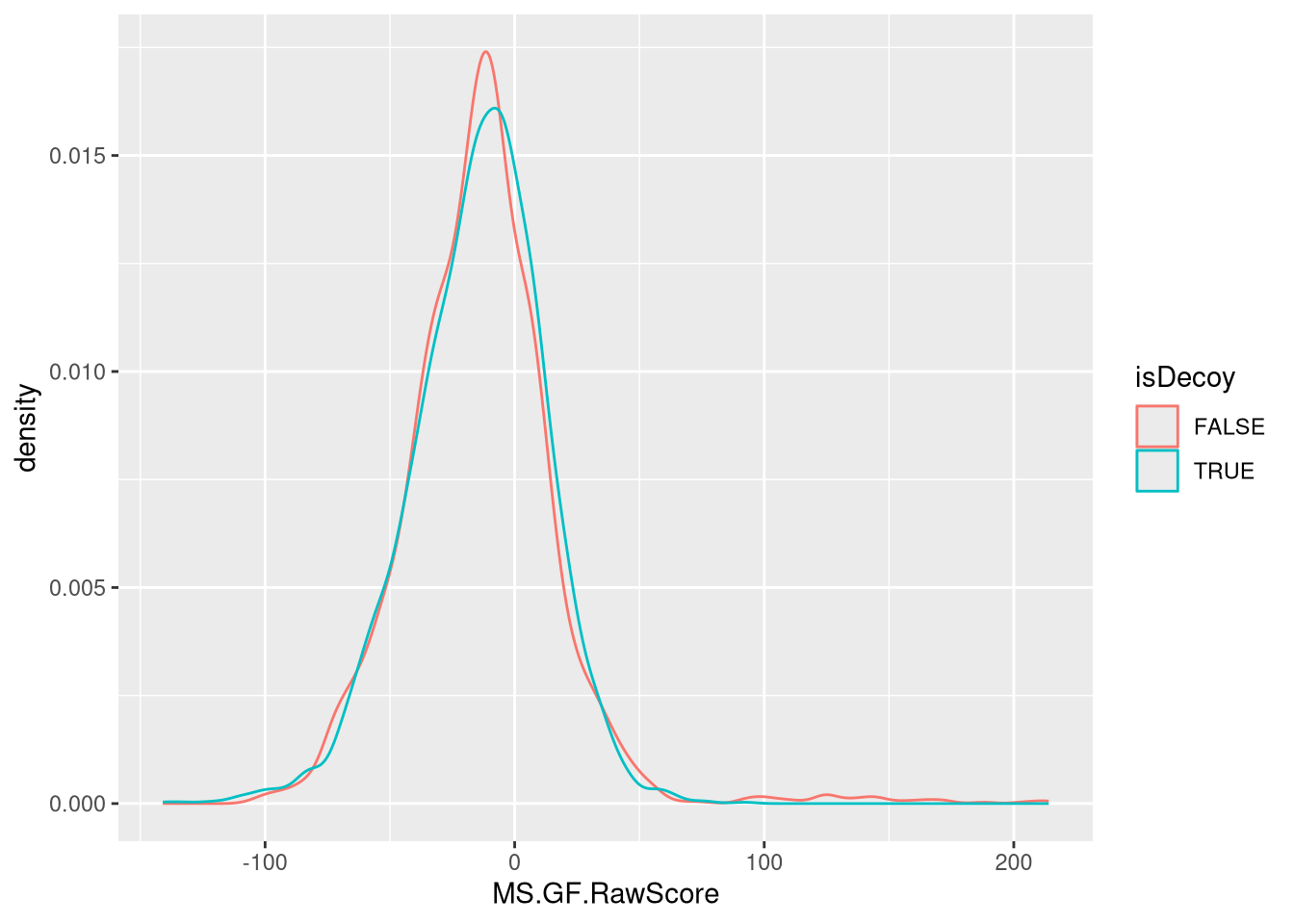
► Question
Compare the distribution of raw identification scores of the decoy and non-decoy hits. Interpret the figure.
► Solution
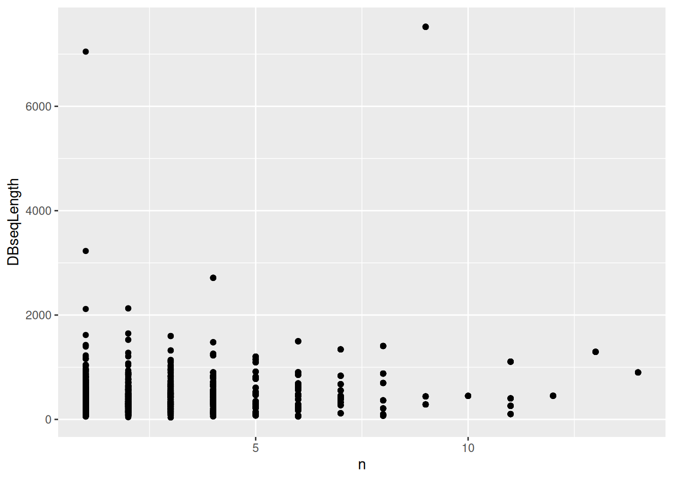
► Question
The tidyverse
tools are fit for data wrangling with identification data. Using the
above identification dataframe, calculate the length of each peptide
(you can use nchar with the peptide sequence sequence) and the
number of peptides for each protein (defined as
DatabaseDescription). Plot the length of the proteins against their
respective number of peptides.
► Solution
If you would like to learn more about how the mzid data are handled by
PSMatch via the mzR and mzID
packages, check out the 7.2 section in the annex.
4.4 Adding identification data to raw data
We are goind to use the sp object created in the previous chapter
and the id_filtered variable generated above.
Identification data (as a DataFrame) can be merged into raw data (as
a Spectra object) by adding new spectra variables to the appropriate
MS2 spectra. Scans and peptide-spectrum matches can be matched by
their spectrum identifers.
► Question
Identify the spectum identifier columns in the sp the id_filtered
variables.
► Solution
We still have several PTMs that are matched to a single spectrum identifier:
##
##    1    2    3    4
## 2630   13    2    1
Let’s look at "controllerType=0 controllerNumber=1 scan=5490", the
has 4 matching PSMs in detail.
## controllerType=0 controllerNumber=1 scan=5490
##                                          1903
id_4 <- id_filtered[id_filtered$spectrumID == "controllerType=0 controllerNumber=1 scan=5490", ] |>
as.data.frame()
id_4## sequence spectrumID
## EH7807.23 KCNQCLKVACTLFYCK controllerType=0 controllerNumber=1 scan=5490
## EH7807.24 KCNQCLKVACTLFYCK controllerType=0 controllerNumber=1 scan=5490
## chargeState rank passThreshold experimentalMassToCharge
## EH7807.23 3 1 TRUE 698.6633
## EH7807.24 3 1 TRUE 698.6633
## calculatedMassToCharge peptideRef modNum isDecoy post pre start end
## EH7807.23 698.3315 Pep453 4 FALSE C K 127 142
## EH7807.24 698.3315 Pep453 4 FALSE C K 127 142
## DatabaseAccess DBseqLength DatabaseSeq DatabaseDescription
## EH7807.23 ECA0668 302 ECA0668 hypothetical protein
## EH7807.24 ECA0668 302 ECA0668 hypothetical protein
## scan.number.s. acquisitionNum
## EH7807.23 5490 5490
## EH7807.24 5490 5490
## spectrumFile
## EH7807.23 TMT_Erwinia_1uLSike_Top10HCD_isol2_45stepped_60min_01-20141210.mzML
## EH7807.24 TMT_Erwinia_1uLSike_Top10HCD_isol2_45stepped_60min_01-20141210.mzML
## idFile MS.GF.RawScore MS.GF.DeNovoScore MS.GF.SpecEValue
## EH7807.23 31c07e307d0acb_7857 -22 79 4.555588e-07
## EH7807.24 31c07e307d0acb_7857 -22 79 4.555588e-07
## MS.GF.EValue MS.GF.QValue MS.GF.PepQValue modPeptideRef
## EH7807.23 1.307689 0.9006211 0.8901099 Pep453
## EH7807.24 1.307689 0.9006211 0.8901099 Pep453
## modName modMass modLocation subOriginalResidue
## EH7807.23 Carbamidomethyl 57.02146 2 <NA>
## EH7807.24 Carbamidomethyl 57.02146 5 <NA>
## subReplacementResidue subLocation
## EH7807.23 <NA> NA
## EH7807.24 <NA> NA
## [ reached 'max' / getOption("max.print") -- omitted 2 rows ]We can see that these 4 PSMs differ by the location of the Carbamidomethyl modification.
##                   modName modLocation
## EH7807.23 Carbamidomethyl           2
## EH7807.24 Carbamidomethyl           5
## EH7807.25 Carbamidomethyl          10
## EH7807.26 Carbamidomethyl          15
Let’s reduce that PSM table before joining it to the Spectra object,
to make sure we have unique one-to-one matches between the raw spectra
and the PSMs.
## Reduced PSM with 2646 rows and 35 columns.
## names(35): sequence spectrumID ... subReplacementResidue subLocation
These two data can thus simply be joined using:
sp <- joinSpectraData(sp, id_filtered,
                      by.x = "spectrumId",
                      by.y = "spectrumID")
spectraVariables(sp)
## [1] "msLevel" "rtime"
## [3] "acquisitionNum" "scanIndex"
## [5] "dataStorage" "dataOrigin"
## [7] "centroided" "smoothed"
## [9] "polarity" "precScanNum"
## [11] "precursorMz" "precursorIntensity"
## [13] "precursorCharge" "collisionEnergy"
## [15] "isolationWindowLowerMz" "isolationWindowTargetMz"
## [17] "isolationWindowUpperMz" "peaksCount"
## [19] "totIonCurrent" "basePeakMZ"
## [21] "basePeakIntensity" "electronBeamEnergy"
## [23] "ionisationEnergy" "lowMZ"
## [25] "highMZ" "mergedScan"
## [27] "mergedResultScanNum" "mergedResultStartScanNum"
## [29] "mergedResultEndScanNum" "injectionTime"
## [31] "filterString" "spectrumId"
## [33] "ionMobilityDriftTime" "scanWindowLowerLimit"
## [35] "scanWindowUpperLimit" "rtime_minute"
## [37] "sequence" "chargeState"
## [39] "rank" "passThreshold"
## [41] "experimentalMassToCharge" "calculatedMassToCharge"
## [43] "peptideRef" "modNum"
## [45] "isDecoy" "post"
## [47] "pre" "start"
## [49] "end" "DatabaseAccess"
## [51] "DBseqLength" "DatabaseSeq"
## [53] "DatabaseDescription" "scan.number.s."
## [55] "acquisitionNum.y" "spectrumFile"
## [57] "idFile" "MS.GF.RawScore"
## [59] "MS.GF.DeNovoScore" "MS.GF.SpecEValue"
## [61] "MS.GF.EValue" "MS.GF.QValue"
## [63] "MS.GF.PepQValue" "modPeptideRef"
## [65] "modName" "modMass"
## [67] "modLocation" "subOriginalResidue"
## [69] "subReplacementResidue" "subLocation"► Question
Verify that the identification data has been added to the correct spectra.
► Solution
4.5 An identification-annotated chromatogram
Now that we have combined raw data and their associated peptide-spectrum matches, we can produce an improved total ion chromatogram, identifying MS1 scans that lead to successful identifications.
The countIdentifications() function is going to tally the number of
identifications (i.e non-missing characters in the sequence spectra
variable) for each scan. In the case of MS2 scans, these will be
either 1 or 0, depending on the presence of a sequence. For MS1 scans,
the function will count the number of sequences for the descendant MS2
scans, i.e. those produced from precursor ions from each MS1 scan.
Below, we see on the second line that 3457 MS2 scans lead to no PSM, while 2546 lead to an identification. Among all MS1 scans, 833 lead to no MS2 scans with PSMs. 30 MS1 scans generated one MS2 scan that lead to a PSM, 45 lead to two PSMs, …
##
##        0    1    2    3    4    5    6    7    8    9   10
##   1  833   30   45   97  139  132   92   42   17    3    1
##   2 3457 2646    0    0    0    0    0    0    0    0    0
These data can also be visualised on the total ion chromatogram:
sp |>
    filterMsLevel(1) |>
    spectraData() |>
    as_tibble() |>
    ggplot(aes(x = rtime,
               y = totIonCurrent)) +
    geom_line(alpha = 0.25) +
    geom_point(aes(colour = ifelse(countIdentifications == 0,
                                   NA, countIdentifications)),
               size = 0.75,
               alpha = 0.5) +
    labs(colour = "Number of ids")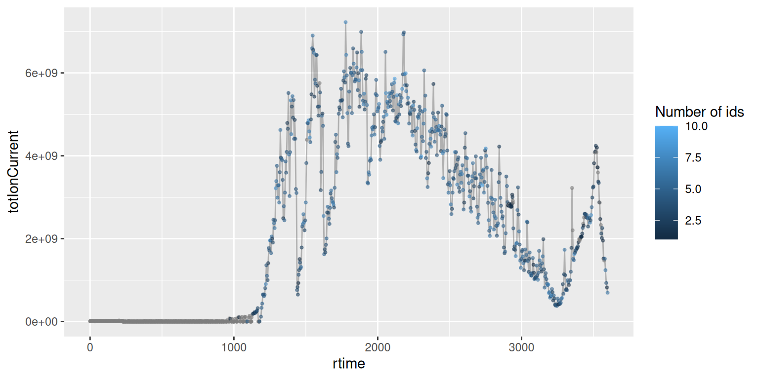
4.6 Visualising peptide-spectrum matches
Let’s choose a MS2 spectrum with a high identification score and plot it.
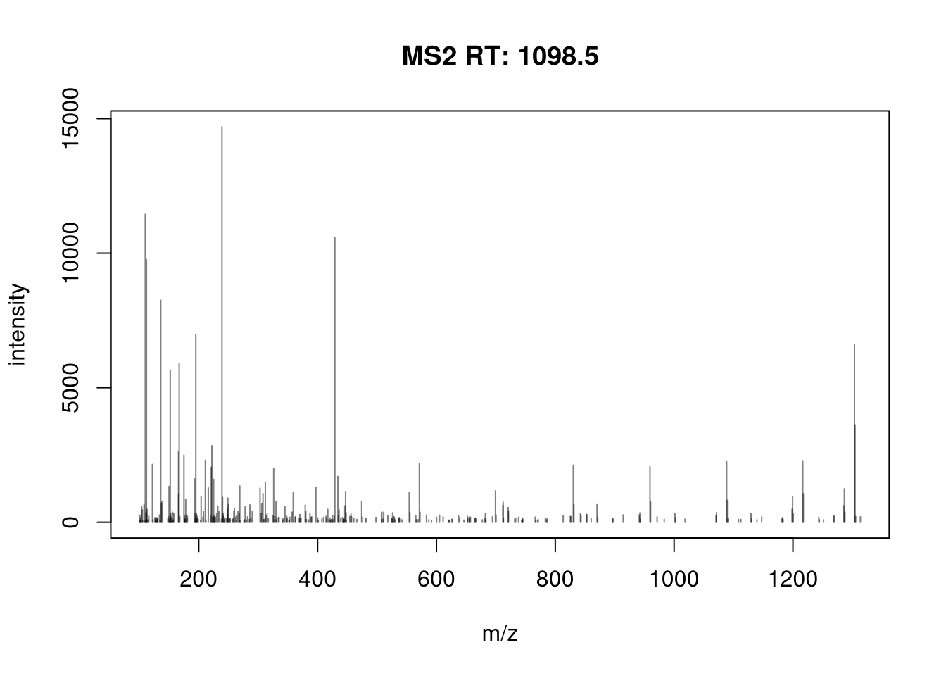
We have seen above that we can add labels to each peak using the
labels argument in plotSpectra(). The labelFragments() function
takes a spectrum as input (that is a Spectra object of length 1) and
annotates its peaks.
## $THSQEEMQHMQR
##   [1] NA    NA    NA    "b1"  NA    NA    NA    NA    NA    NA    NA    NA
##  [13] NA    NA    NA    NA    NA    NA    NA    NA    NA    NA    NA    NA
##  [25] NA    NA    NA    NA    NA    NA    NA    NA    NA    NA    NA    NA
##  [37] NA    NA    NA    NA    NA    NA    NA    "y1_" NA    NA    NA    NA
##  [49] NA    "y1"  NA    NA    NA    NA    NA    NA    NA    NA    NA    NA
##  [61] NA    NA    NA    NA    NA    NA    NA    NA    NA    NA    NA    NA
##  [73] NA    NA    NA    NA    NA    NA    NA    NA    NA    NA    NA    NA
##  [85] NA    NA    "b2"  NA    NA    NA    NA    NA    NA    NA    NA    NA
##  [97] NA    NA    NA    NA
##  [ reached 'max' / getOption("max.print") -- omitted 227 entries ]
##
## attr(,"group")
## [1] 1
It can be directly used with plotSpectra():
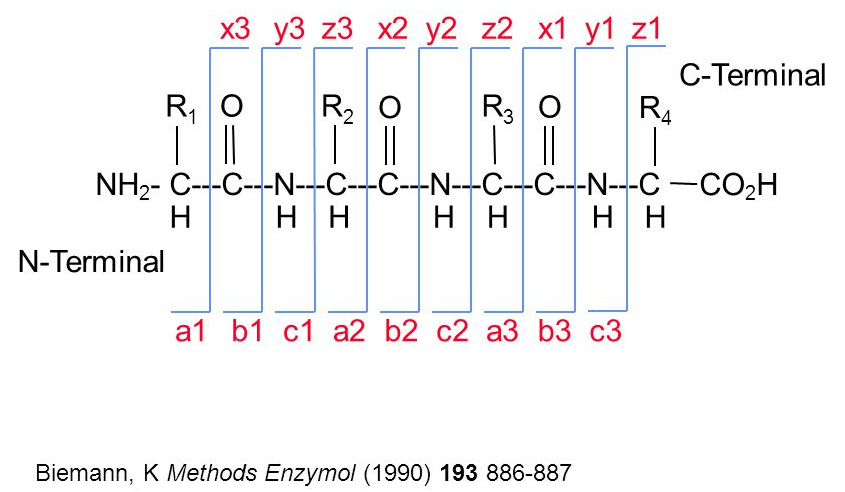
When a precursor peptide ion is fragmented in a CID cell, it breaks at specific bonds, producing sets of peaks (a, b, c and x, y, z) that can be predicted.
(#fig:frag_img)Peptide fragmentation.
The annotation of spectra is obtained by simulating fragmentation of a peptide and matching observed peaks to fragments:
## [1] "THSQEEMQHMQR"## Fixed modifications used: C=57.02146
## Variable modifications used: None## mz ion type pos z seq peptide
## 1 102.0550 b1 b 1 1 T THSQEEMQHMQR
## 2 239.1139 b2 b 2 1 TH THSQEEMQHMQR
## 3 326.1459 b3 b 3 1 THS THSQEEMQHMQR
## 4 454.2045 b4 b 4 1 THSQ THSQEEMQHMQR
## 5 583.2471 b5 b 5 1 THSQE THSQEEMQHMQR
## 6 712.2897 b6 b 6 1 THSQEE THSQEEMQHMQR
## 7 843.3301 b7 b 7 1 THSQEEM THSQEEMQHMQR
## 8 971.3887 b8 b 8 1 THSQEEMQ THSQEEMQHMQR
## 9 1108.4476 b9 b 9 1 THSQEEMQH THSQEEMQHMQR
## 10 1239.4881 b10 b 10 1 THSQEEMQHM THSQEEMQHMQR
## 11 1367.5467 b11 b 11 1 THSQEEMQHMQ THSQEEMQHMQR
## 12 175.1190 y1 y 1 1 R THSQEEMQHMQR
## 13 303.1775 y2 y 2 1 QR THSQEEMQHMQR
## 14 434.2180 y3 y 3 1 MQR THSQEEMQHMQR
## [ reached 'max' / getOption("max.print") -- omitted 44 rows ]Note that the plotSpectraPTM() from the PSMatch
package offers
improved visualisation:
- The function nadds the annotated peptides sequence on the plot with the respective b and y ions and the deviation between observed and calculated fragment masses.

- It can also display, as its name implies, multi-panel plots for peptides with variable modifications.
4.7 Comparing spectra
The compareSpectra() function can be used to compare spectra (by default,
computing the normalised dot product).
► Question
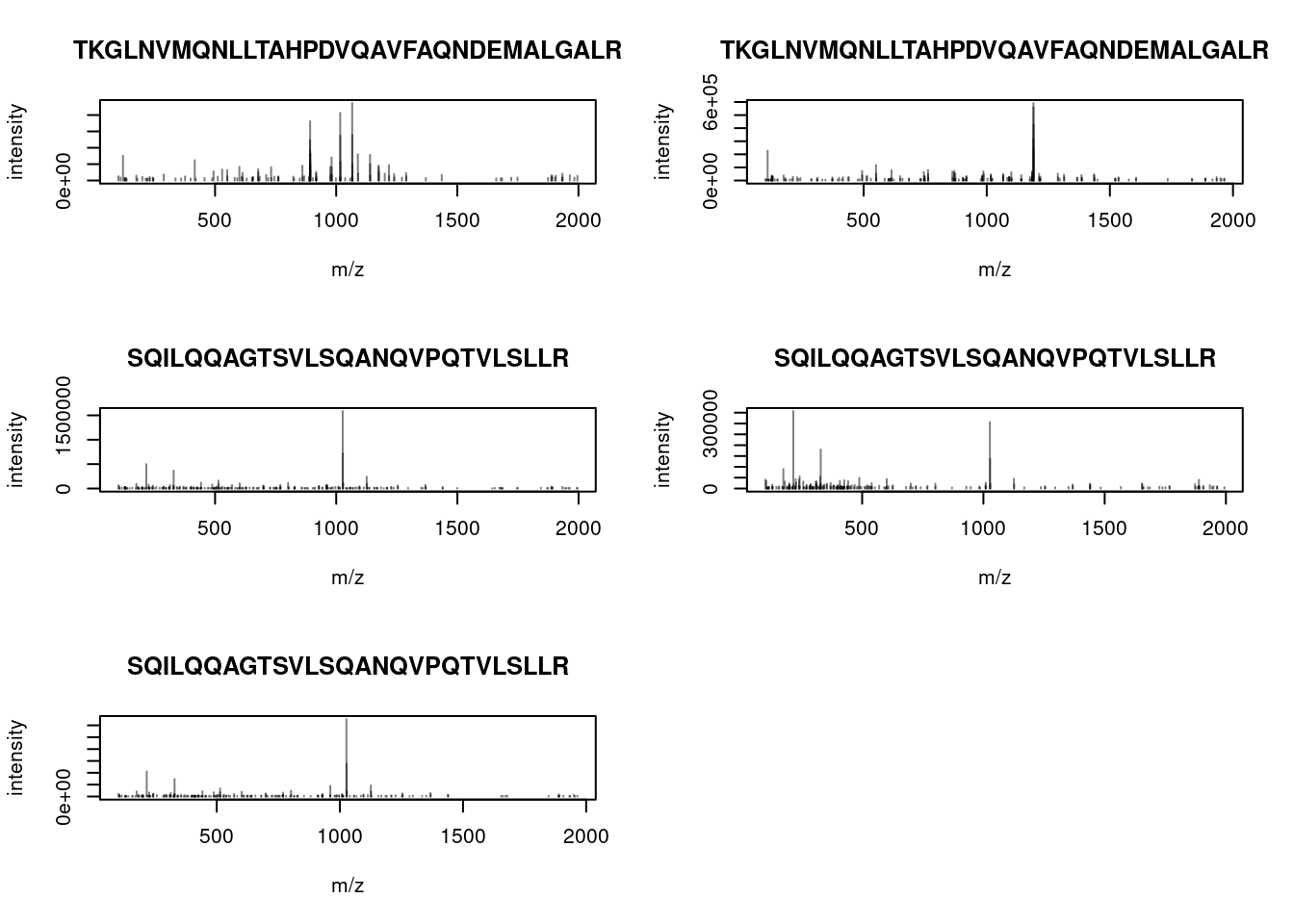
- Create a new
Spectraobject containing the MS2 spectra with sequences"SQILQQAGTSVLSQANQVPQTVLSLLR"and"TKGLNVMQNLLTAHPDVQAVFAQNDEMALGALR".
► Solution
► Question
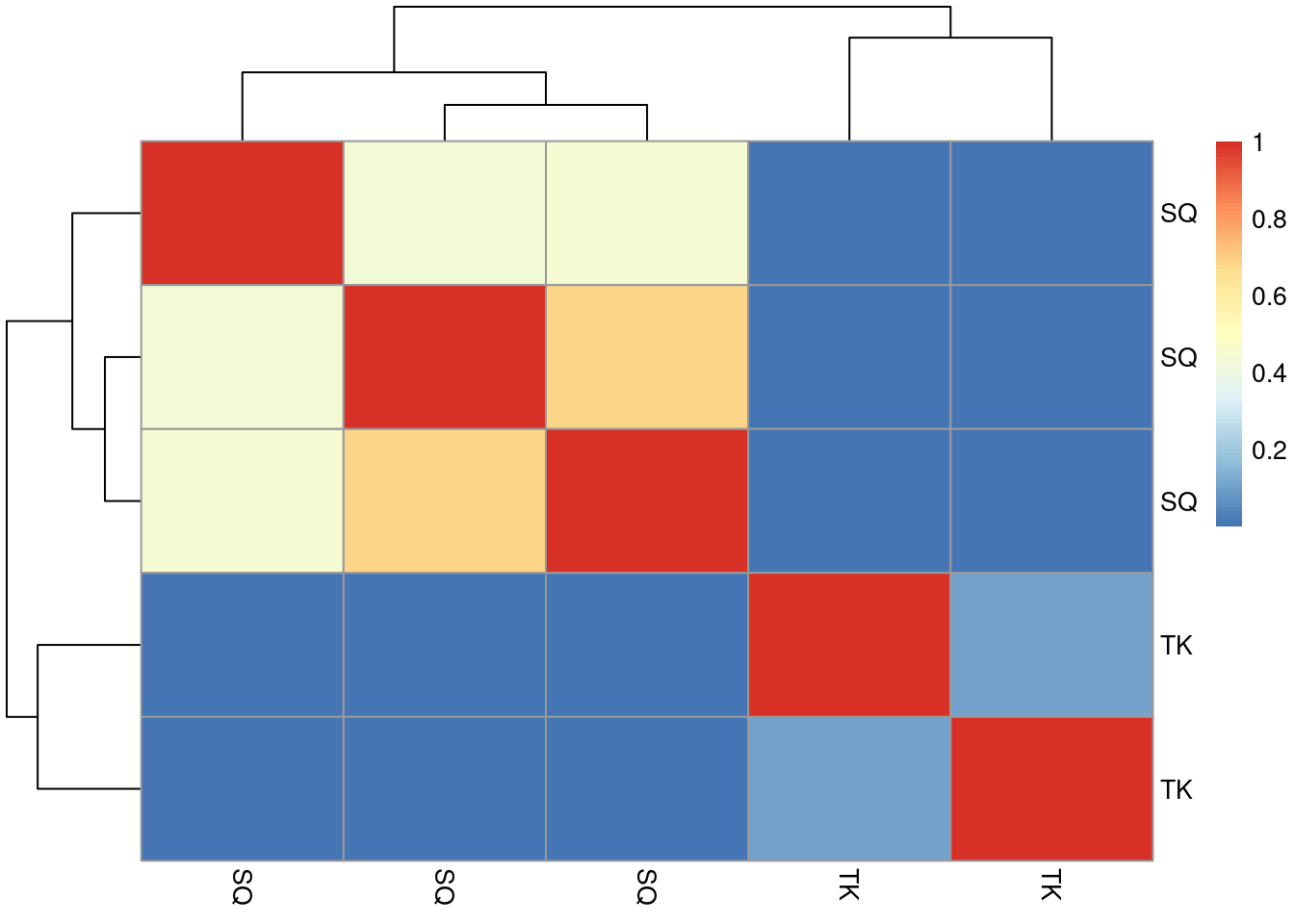
- Calculate the 5 by 5 similarity
matrix between all spectra using
compareSpectra. See the?Spectraman page for details. Draw a heatmap of that matrix.
► Solution
► Question
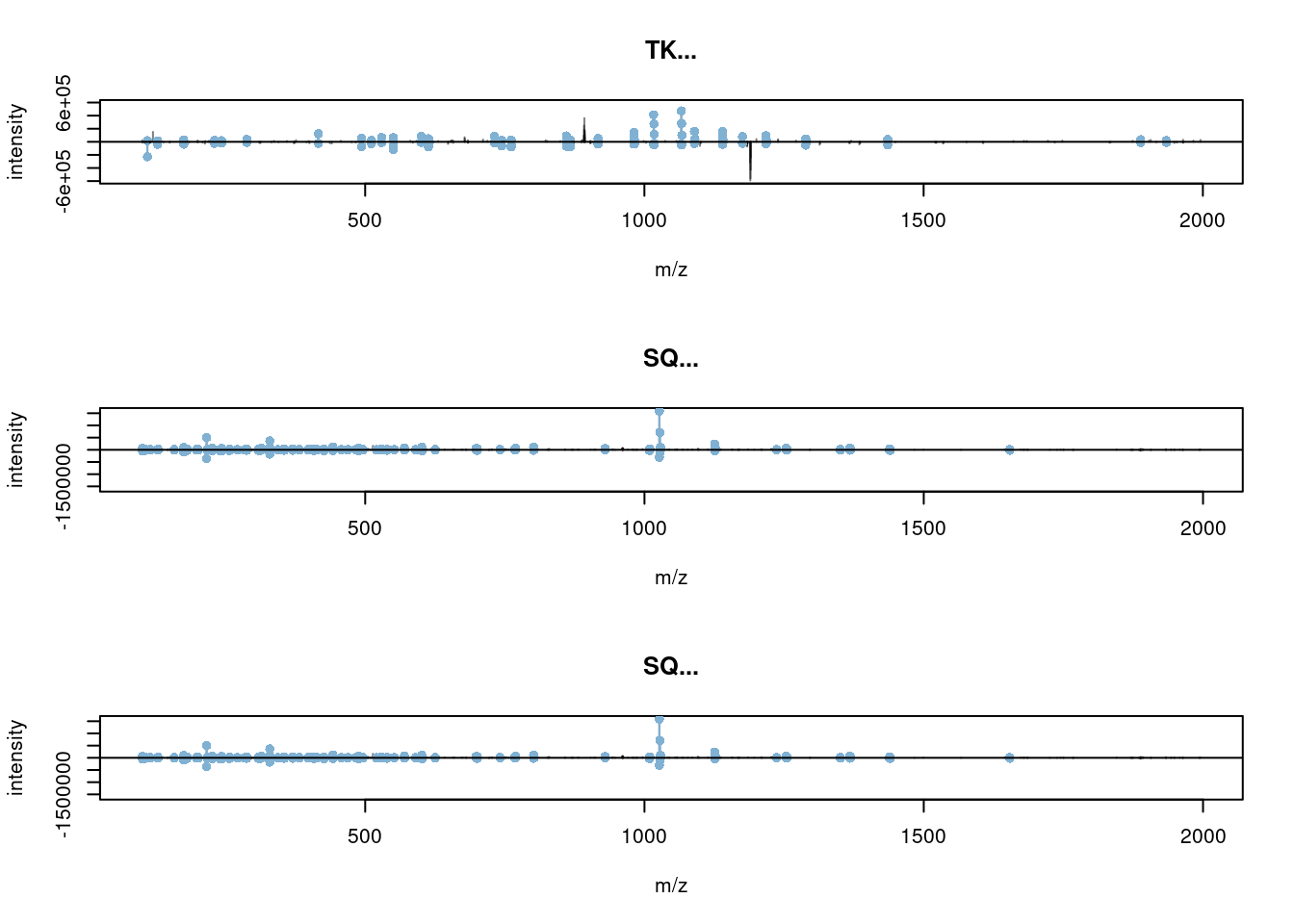
- Compare the spectra with the plotting function seen previously.
► Solution

4.8 Reading and processing protein sequences
It can sometimes be necessary to do some protein sequence processing in R, for compute peptides for a set of proteins of interest. Let’s start by downloading the fasta sequence file from the PXD000001 experiment.
## Loading PXD000001 from cache.## Project PXD000001 files (11):
## [remote] F063721.dat
## [local] F063721.dat-mztab.txt
## [remote] PRIDE_Exp_Complete_Ac_22134.xml.gz
## [remote] PRIDE_Exp_mzData_Ac_22134.xml.gz
## [remote] PXD000001_mztab.txt
## [remote] README.txt
## [local] TMT_Erwinia_1uLSike_Top10HCD_isol2_45stepped_60min_01-20141210.mzML
## [remote] TMT_Erwinia_1uLSike_Top10HCD_isol2_45stepped_60min_01-20141210.mzXML
## [remote] TMT_Erwinia_1uLSike_Top10HCD_isol2_45stepped_60min_01.mzXML
## [remote] TMT_Erwinia_1uLSike_Top10HCD_isol2_45stepped_60min_01.raw
## ...## Warning in rep(as.integer(len), length = length(str)): partial argument match
## of 'length' to 'length.out'## Loading erwinia_carotovora.fasta from cache.## [1] "/home/lgatto/.cache/R/rpx/4cdea72b57ef5_erwinia_carotovora.fasta"The fasta file can be read into R as a dedicated AAStringSet from
the Biostrings package, that can be used to
very efficiently manage DNA, RNA and protein sequence.
## AAStringSet object of length 4499:
##        width seq                                            names
##    [1]   147 MADITLISGSTLGSAEYVAEHL...QHQIPEDPAEEWLGSWVNLLK ECA0001 putative ...
##    [2]   153 VAEIYQIDNLDRGILSALMENA...EIQSTETLISLQNPIMRTIAP ECA0002 AsnC-fami...
##    [3]   330 MKKQYIEKQQQISFVKSFFSSQ...IGQVQCGVWPQPLRESVSGLL ECA0003 putative ...
##    [4]   492 MITLESLEMLLSIDENELLDDL...WRFDTGLKSRLMRRWQHGKAY ECA0004 conserved...
##    [5]   499 MRQTAALAERISRLSHALEHGL...AKIEASLQQVAEQIQQSEQQD ECA0005 conserved...
##    ...   ... ...
## [4495]   634 MSDKIIHLTDDSFDTDVLKADG...RRKVDPLRVFASDMARRLELL trx-rv3790 trx-rv...
## [4496]    93 MTKMNNKARRTARELKHLGASI...RELRDEFPMGYLGDYKDDDDK TimBlower TimBlower
## [4497]   309 MFSNLSKRWAQRTLSKSFYSTA...KFKWAGIKTRKFVFNPPKPRK sp|P07143|CY1_YEA...
## [4498]   231 FPTDDDDKIVGGYTCAANSIPY...PGVYTKVCNYVNWIQQTIAAN sp|P00761|TRYP_PI...
## [4499]   269 GVSGSCNIDVVCPEGNGHRDVI...DAAGTGAQFIDGLDSTGTPPV sp|Q7M135|LYSC_LY...
Finally, the cleaver package can be used to cleave protein sequences using any of the many proteases. Below, we’ll use trypsin without any miscleavages.
## AAStringSetList of length 4499
## [["ECA0001 putative flavoprotein (initiation of chromosome replication)"]] MA...
## [["ECA0002 AsnC-family transcriptional regulator"]] VAEIYQIDNLDR ... TIAP
## [["ECA0003 putative asparagine synthetase A"]] MK K ... ESVSGLL
## [["ECA0004 conserved hypothetical protein"]] MITLESLEMLLSIDENELLDDLVVTLMATPQL...
## [["ECA0005 conserved hypothetical protein"]] MR ... IEASLQQVAEQIQQSEQQD
## [["ECA0006 potassium uptake protein"]] MSSEHK R ... AADQFEIPPNR LIELGIQVEI
## [["ECA0007 two-component system sensor kinase"]] MNR LSLR ... VTFTNQPEGGLIVSVNW
## [["ECA0008 two-component system response regulator."]] MR ... TVHGVGYILGDAP
## [["ECA0009 putative exported protein"]] MK K ... QIR L
## [["ECA0010 high affinity ribose transport protein"]] MK ... SGECSPYANVILCAGVTF
## ...
## <4489 more elements>
The resulting AAStringSetList contains the one AAStringSet
containing peptides sequences for each of the 4499
proteins.
## AAStringSet object of length 7:
##     width seq
## [1]    28 MADITLISGSTLGSAEYVAEHLAELLEK
## [2]    39 DNFSTEILHGPTLDALPESGIWLVVTSTHGAGEFPDNLK
## [3]    26 ALFEQLEQQKPDLSQVNFGAIGIGSK
## [4]    14 EYDTFCGAIQTADR
## [5]     8 LLAQLGAK
## [6]     1 R
## [7]    31 IGEILEIDITQHQIPEDPAEEWLGSWVNLLK
It is also possible to repeat the above step to generate a decoy
database by reversing the protein AAStringSet object:
## AAStringSet object of length 4499:
##        width seq                                            names
##    [1]   147 KLLNVWSGLWEEAPDEPIQHQT...HEAVYEASGLTSGSILTIDAM ECA0001 putative ...
##    [2]   153 PAITRMIPNQLSILTETSQIED...NEMLASLIGRDLNDIQYIEAV ECA0002 AsnC-fami...
##    [3]   330 LLGSVSERLPQPWVGCQVQGIH...SSFFSKVFSIQQQKEIYQKKM ECA0003 putative ...
##    [4]   492 YAKGHQWRRMLRSKLGTDFRWI...DDLLENEDISLLMELSELTIM ECA0004 conserved...
##    [5]   499 DQQESQQIQEAVQQLSAEIKAL...GHELAHSLRSIREALAATQRM ECA0005 conserved...
##    ...   ... ...
## [4495]   634 LLELRRAMDSAFVRLPDVKRRV...DAKLVDTDFSDDTLHIIKDSM trx-rv3790 trx-rv...
## [4496]    93 KDDDDKYDGLYGMPFEDRLERY...SAGLHKLERATRRAKNNMKTM TimBlower TimBlower
## [4497]   309 KRPKPPNFVFKRTKIGAWKFKK...TSYFSKSLTRQAWRKSLNSFM sp|P07143|CY1_YEA...
## [4498]   231 NAAITQQIWNVYNCVKTYVGPK...PISNAACTYGGVIKDDDDTPF sp|P00761|TRYP_PI...
## [4499] 269 VPPTGTSDLGDIFQAGTGAADL...VDRHGNGEPCVVDINCSGSVG sp|Q7M135|LYSC_LY...## 147-letter AAString object
## seq: MADITLISGSTLGSAEYVAEHLAELLEKDNFSTEIL...LGAKRIGEILEIDITQHQIPEDPAEEWLGSWVNLLK## 147-letter AAString object
## seq: KLLNVWSGLWEEAPDEPIQHQTIDIELIEGIRKAGL...LIETSFNDKELLEALHEAVYEASGLTSGSILTIDAM
4.9 Exploration and Assessment of Identifications using MSnID
The MSnID package extracts MS/MS ID data from mzIdentML (leveraging
the mzID package) or text files. After collating the search results
from multiple datasets it assesses their identification quality and
optimises filtering criteria to achieve the maximum number of
identifications while not exceeding a specified false discovery
rate. It also contains a number of utilities to explore the MS/MS
results and assess missed and irregular enzymatic cleavages, mass
measurement accuracy, etc.
4.9.1 Step-by-step work-flow
Let’s reproduce parts of the analysis described the MSnID
vignette. You can explore more with
The MSnID package can be used for post-search filtering
of MS/MS identifications. One starts with the construction of an
MSnID object that is populated with identification results that can
be imported from a data.frame or from mzIdenML files. Here, we
will use the example identification data provided with the package.
## [1] "c_elegans.mzid.gz"We start by loading the package, initialising the MSnID object, and
add the identification result from our mzid file (there could of
course be more than one).
## Note, the anticipated/suggested columns in the
## peptide-to-spectrum matching results are:
## -----------------------------------------------
## accession
## calculatedMassToCharge
## chargeState
## experimentalMassToCharge
## isDecoy
## peptide
## spectrumFile
## spectrumID## Loaded cached data## MSnID object
## Working directory: "."
## #Spectrum Files: 1
## #PSMs: 12263 at 36 % FDR
## #peptides: 9489 at 44 % FDR
## #accessions: 7414 at 76 % FDRPrinting the MSnID object returns some basic information such as
- Working directory.
- Number of spectrum files used to generate data.
- Number of peptide-to-spectrum matches and corresponding FDR.
- Number of unique peptide sequences and corresponding FDR.
- Number of unique proteins or amino acid sequence accessions and corresponding FDR.
The package then enables to define, optimise and apply filtering based for example on missed cleavages, identification scores, precursor mass errors, etc. and assess PSM, peptide and protein FDR levels. To properly function, it expects to have access to the following data
## [1] "accession"                "calculatedMassToCharge"
## [3] "chargeState"              "experimentalMassToCharge"
## [5] "isDecoy"                  "peptide"
## [7] "spectrumFile"             "spectrumID"
which are indeed present in our data:
##  [1] "spectrumID"                "scan number(s)"
##  [3] "acquisitionNum"            "passThreshold"
##  [5] "rank"                      "calculatedMassToCharge"
##  [7] "experimentalMassToCharge"  "chargeState"
##  [9] "MS-GF:DeNovoScore"         "MS-GF:EValue"
## [11] "MS-GF:PepQValue"           "MS-GF:QValue"
## [13] "MS-GF:RawScore"            "MS-GF:SpecEValue"
## [15] "AssumedDissociationMethod" "IsotopeError"
## [17] "isDecoy"                   "post"
## [19] "pre"                       "end"
## [21] "start"                     "accession"
## [23] "length"                    "description"
## [25] "pepSeq"                    "modified"
## [27] "modification"              "idFile"
## [29] "spectrumFile"              "databaseFile"
## [31] "peptide"
Here, we summarise a few steps and redirect the reader to the package’s vignette for more details:
4.9.2 Analysis of peptide sequences
Cleaning irregular cleavages at the termini of the peptides and
missing cleavage site within the peptide sequences. The following two
function calls create the new numMisCleavages and numIrregCleavages
columns in the MSnID object
4.9.3 Trimming the data
Now, we can use the apply_filter function to effectively apply
filters. The strings passed to the function represent expressions that
will be evaluated, thus keeping only PSMs that have 0 irregular
cleavages and 2 or less missed cleavages.
msnid <- apply_filter(msnid, "numIrregCleavages == 0")
msnid <- apply_filter(msnid, "numMissCleavages <= 2")
show(msnid)
## MSnID object
## Working directory: "."
## #Spectrum Files: 1
## #PSMs: 7838 at 17 % FDR
## #peptides: 5598 at 23 % FDR
## #accessions: 3759 at 53 % FDR4.9.4 Parent ion mass errors
Using "calculatedMassToCharge" and "experimentalMassToCharge", the
mass_measurement_error function calculates the parent ion mass
measurement error in parts per million.
##       Min.    1st Qu.     Median       Mean    3rd Qu.       Max.
## -2184.0640    -0.6992     0.0000    17.6146     0.7511  2012.5178
We then filter any matches that do not fit the +/- 20 ppm tolerance
msnid <- apply_filter(msnid, "abs(mass_measurement_error(msnid)) < 20")
summary(mass_measurement_error(msnid))
## Min. 1st Qu. Median Mean 3rd Qu. Max.
## -19.7797 -0.5866 0.0000 -0.2970 0.5713 19.67584.9.5 Filtering criteria
Filtering of the identification data will rely on
- -log10 transformed MS-GF+ Spectrum E-value, reflecting the goodness of match between experimental and theoretical fragmentation patterns
- the absolute mass measurement error (in ppm units) of the parent ion
4.9.6 Setting filters
MS2 filters are handled by a special MSnIDFilter class objects, where
individual filters are set by name (that is present in names(msnid))
and comparison operator (>, <, = , …) defining if we should retain
hits with higher or lower given the threshold and finally the
threshold value itself.
filtObj <- MSnIDFilter(msnid)
filtObj$absParentMassErrorPPM <- list(comparison="<", threshold=10.0)
filtObj$msmsScore <- list(comparison=">", threshold=10.0)
show(filtObj)
## MSnIDFilter object
## (absParentMassErrorPPM < 10) & (msmsScore > 10)We can then evaluate the filter on the identification data object, which returns the false discovery rate and number of retained identifications for the filtering criteria at hand.
##           fdr    n
## PSM         0 3807
## peptide     0 2455
## accession   0 1009
4.9.7 Filter optimisation
Rather than setting filtering values by hand, as shown above, these can be set automatically to meet a specific false discovery rate.
filtObj.grid <- optimize_filter(filtObj, msnid, fdr.max=0.01,
                                method="Grid", level="peptide",
                                n.iter=500)
show(filtObj.grid)
## MSnIDFilter object
## (absParentMassErrorPPM < 3) & (msmsScore > 7.4)## fdr n
## PSM 0.004097561 5146
## peptide 0.006447651 3278
## accession 0.021996616 1208Filters can eventually be applied (rather than just evaluated) using
the apply_filter function.
## MSnID object
## Working directory: "."
## #Spectrum Files:  1
## #PSMs: 5146 at 0.41 % FDR
## #peptides: 3278 at 0.64 % FDR
## #accessions: 1208 at 2.2 % FDR
And finally, identifications that matched decoy and contaminant protein sequences are removed
msnid <- apply_filter(msnid, "isDecoy == FALSE")
msnid <- apply_filter(msnid, "!grepl('Contaminant',accession)")
show(msnid)
## MSnID object
## Working directory: "."
## #Spectrum Files: 1
## #PSMs: 5117 at 0 % FDR
## #peptides: 3251 at 0 % FDR
## #accessions: 1179 at 0 % FDR
4.9.8 Export MSnID data
The resulting filtered identification data can be exported to a
data.frame (or to a dedicated MSnSet data structure from the
MSnbase package) for quantitative MS data, described below, and
further processed and analysed using appropriate statistical tests.
##   spectrumID scan number(s) acquisitionNum passThreshold rank
## 1 index=7151           8819           7151          TRUE    1
## 2 index=8520          10419           8520          TRUE    1
##   calculatedMassToCharge experimentalMassToCharge chargeState MS-GF:DeNovoScore
## 1               1270.318                 1270.318           3               287
## 2               1426.737                 1426.739           3               270
##   MS-GF:EValue MS-GF:PepQValue MS-GF:QValue MS-GF:RawScore MS-GF:SpecEValue
## 1 1.709082e-24               0            0            239     1.007452e-31
## 2 3.780745e-24               0            0            230     2.217275e-31
##   AssumedDissociationMethod IsotopeError isDecoy post pre end start accession
## 1                       CID            0   FALSE    A   K 283   249   CE02347
## 2                       CID            0   FALSE    A   K 182   142   CE07055
##   length
## 1    393
## 2    206
##                                                                                                                           description
## 1 WBGene00001993; locus:hpd-1; 4-hydroxyphenylpyruvate dioxygenase; status:Confirmed; UniProt:Q22633; protein_id:CAA90315.1; T21C12.2
## 2           WBGene00001755; locus:gst-7; glutathione S-transferase; status:Confirmed; UniProt:P91253; protein_id:AAB37846.1; F11G11.2
##                                      pepSeq modified modification
## 1       AISQIQEYVDYYGGSGVQHIALNTSDIITAIEALR    FALSE         <NA>
## 2 SAGSGYLVGDSLTFVDLLVAQHTADLLAANAALLDEFPQFK    FALSE         <NA>
##              idFile                                   spectrumFile
## 1 c_elegans.mzid.gz c_elegans_A_3_1_21Apr10_Draco_10-03-04_dta.txt
## 2 c_elegans.mzid.gz c_elegans_A_3_1_21Apr10_Draco_10-03-04_dta.txt
##               databaseFile                                       peptide
## 1 ID_004174_E48C5B52.fasta       K.AISQIQEYVDYYGGSGVQHIALNTSDIITAIEALR.A
## 2 ID_004174_E48C5B52.fasta K.SAGSGYLVGDSLTFVDLLVAQHTADLLAANAALLDEFPQFK.A
##   numIrregCleavages numMissCleavages msmsScore absParentMassErrorPPM
## 1                 0                0  30.99678             0.3843772
## 2                 0                0  30.65418             1.3689451
## [ reached 'max' / getOption("max.print") -- omitted 4 rows ]Page built: 2026-06-26 using R version 4.6.0 (2026-04-24)