
mzTab-M file format: import-export of mzTab-M 2.1 files from SummarizedExperiment
2026-09-11
Source:vignettes/generation_of_mzTabM_file.qmd
Introduction
mzTab-M is a lightweight, tab-delimited file format for reporting quantitative results from metabolomics/lipidomics experiments. This format aims to give local LIMS systems and MS metabolomics repositories a simple way to share and combine basic information.
This document shows how to export and import a mzTab-M file into R via the RmzTabM Bioconductor package, which provides the API and core functionality to read and write files in this format.
The RmzTabM package supports mzTab-M version 2.1.
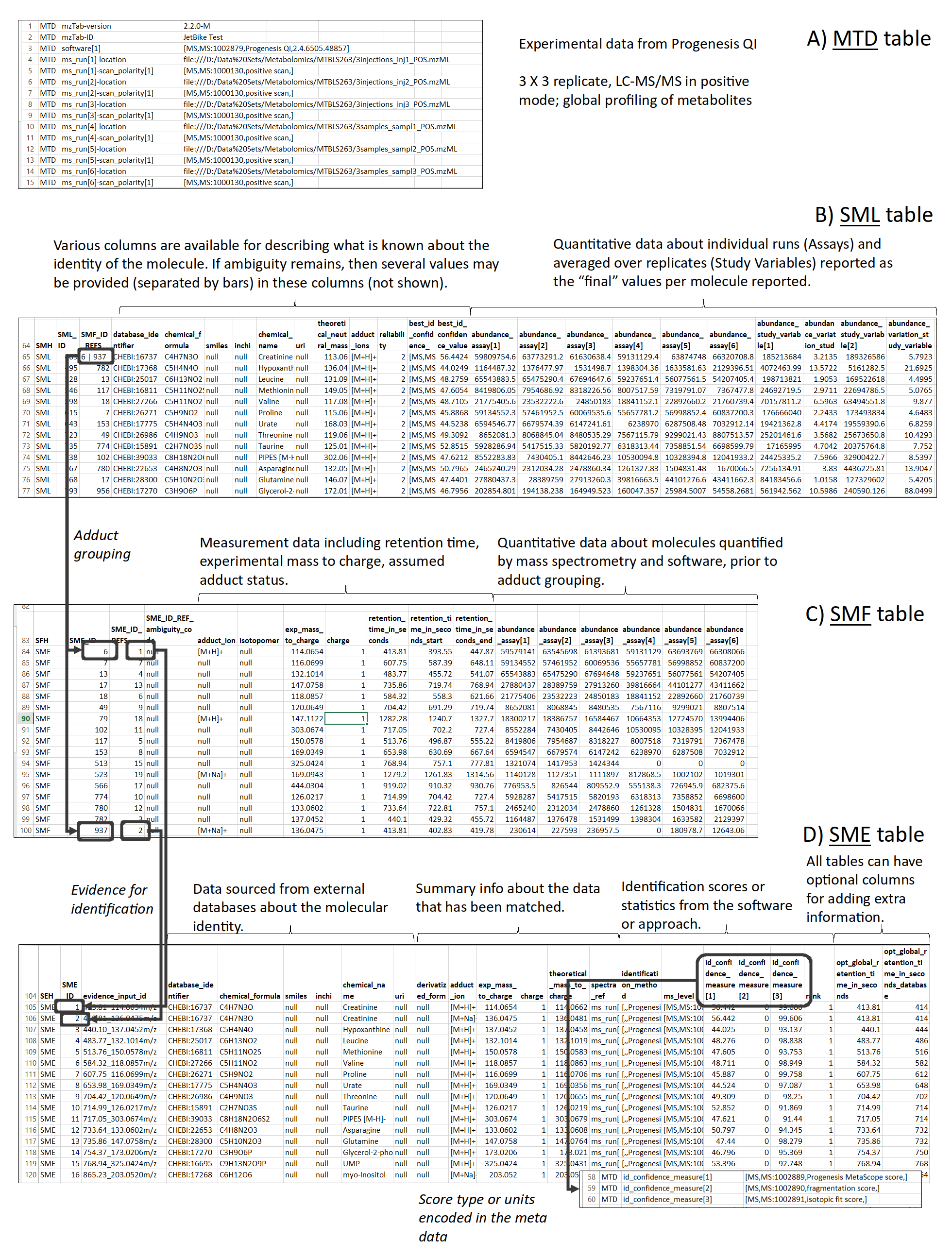
For a general overview of the mzTab-M format see this figure.

For a description of the mzTab-M format and the set of mandatory and optional fields refer to the official format definition.
General information on the mzTab-M format
The mzTab-M format consists of four cross-referenced data tables: metadata (MTD), Small Molecule (SML), Small Molecule Feature (SMF) and the Small Molecule Evidence (SME). The MTD section is supposed to contain all experiment and measurement relevant information. The SML section contains the final results of an analysis that should be reported, i.e., the (annotated) molecules and their respective abundances. The SMF section contains information on the measured (LC-MS) features and their abundance values. The SME section contains information on the annotation process (and reliability) of the molecules reported in the SML section. The SML is supposed to be a subset of the SMF table. The structure and relationship between rows in these different tables is defined by the mzTab-M standard and follows strict rules. All mzTab-M files are validated using either the online or local Java validator to ensure compliance. In RmzTabM, this validation is executed locally via the offline Java tool.
Package
## Data Import and handling
library(alabaster.base)
library(MsIO)
library(xcms)
library(SummarizedExperiment)
Export of a SummarizedExperiment to mzTab-M
Data import
In this document we export the preprocessed data set used in the Metabonaut end-to-end metabolomics data workflow in mzTab-M format. The original MS data is available in the Metabolights repository with accession MTBLS8735. After collecting all necessary experimental metadata, we export this result object as a mzTab-M file with only the metadata and the small feature abundances (MTD+SMF).
## load preprocessed dataset
se <- readObject(system.file("extdata", "preprocessed_res",
                             package = "Metabonaut"))
Creation of the MzTabM object
The RmzTabM package defines a MzTabM() convenience function to create a mzTab-M file from a SummarizedExperiment object. Information provided in such objects is automatically converted and formatted into content for the right mzTab-M section. The user simply needs to define the columns containing information for the various mzTab-M fields and a mzTab-M is compiled. The resulting MzTabM object should then be manually completed adding eventually missing data.
Define missing data set’s metadata (MTD)
Comprehensive data set descriptions and metadata are important to enable re-use of the data and follow FAIR principles. The mzTab-M format has stringent requirements for mandatory fields and their format. Most of the fields are controlled vocabulary (CV) parameters and the PSI Mass Spectrometry Controlled Vocabulary (PSI-MS) is the primary CV used to annotate mass spectrometry-specific fields in mzTab-M. It was built collaboratively by MS software vendors and academic groups working in mass spectrometry and MS informatics. The CV is community-maintained: new terms can be requested through the PSI-MS mailing list. For more details see the mzTab-M specification, section 4.2 “The PSI Mass Spectrometry Controlled Vocabulary (CV)”.
We need to add/adapt some columns of the SummarizedExperiment’s colData() to complete or match the expected format:
- use a CV param for species:
"[NCBITaxon, NCBITaxon:9606, Homo sapiens, ]" - use a CV param for blood plasma:
"[BTO, BTO:0000131, blood plasma, ]" - use a CV param for blood serum:
"[BTO, BTO:0000133, blood serum, ]" - add polarity information.
- assign the same name to all sample pools.
- Add the MS instrument.
colData(se)$species <- "[NCBITaxon, NCBITaxon:9606, Homo sapiens, ]"

colData(se)$tissue <- "[BTO, BTO:0000131, blood plasma, ]"
colData(se)$tissue[colData(se)$blood_sample_type == "blood serum"] <-
              "[BTO, BTO:0000133, blood serum, ]"

colData(se)$polarity <- "positive"

colData(se)$sample_name[grep("POOL", colData(se)$sample_name)] <- "POOL"

colData(se)$instrument <- "1"
Note
ℹ️ ideally, CV parameters should be used as much as possible to ensure a standardized description of the data. The EMBL-EBI Ontology Lookup Service can be used to find ontology terms (CV parameters) for various controlled vocabularies.
Define Metadata (MTD) section
Now we can use the previous information to compile the data set’s metadata. To this end we define the column names in the SummarizedExperiment’s colData() that contain information for the sample, measurement run and assay mzTab-M fields. This mapping of mzTab-M fields to column names can be defined with the sampleCols(), msRunCols() and assayCols() helper functions, respectively. In our example we use the content of column "sample_name" as the mzTab-M sample name. Content from the colData() columns "species", "tissue" and "sample_type" is used for mzTab-M sample fields species`, tissue and sample_type.
## define mapping of `colData()` column names to mzTab-M sample fields
scols <- sampleCols(sample = "sample_name", species = "species",
                    tissue = "tissue", sample_type = "sample_type")
Similarly we specify columns from the same colData() with information on individual MS runs (and assays):
The column "derived_spectra_data_file" contains the MS data file name which we use to define both the MS runs and assays (assuming thus a 1:1 mapping between them).
colData(se)$derived_spectra_data_file [1] "FILES/MS_QC_POOL_1_POS.mzML" "FILES/MS_A_POS.mzML"
[3] "FILES/MS_B_POS.mzML" "FILES/MS_QC_POOL_2_POS.mzML"
[5] "FILES/MS_C_POS.mzML" "FILES/MS_D_POS.mzML"
[7] "FILES/MS_QC_POOL_3_POS.mzML" "FILES/MS_E_POS.mzML"
[9] "FILES/MS_F_POS.mzML" "FILES/MS_QC_POOL_4_POS.mzML"At last we define also the study variables of the experiment. These can be technical characteristics or phenotype(s) of the samples. The present experiment consists of plasma samples of individuals with or without a cardiovascular disease (CVD) and repeated measurements of an external (serum) sample pool that was used as quality control sample. These are defined in colData() columns "blood_sample_type", "age" and "phenotype".
| blood_sample_type | phenotype | age | |
|---|---|---|---|
| MS_QC_POOL_1_POS.mzML | blood serum | QC | NA |
| MS_A_POS.mzML | blood plasma | CVD | 53 |
| MS_B_POS.mzML | blood plasma | CTR | 30 |
| MS_QC_POOL_2_POS.mzML | blood serum | QC | NA |
| MS_C_POS.mzML | blood plasma | CTR | 66 |
| MS_D_POS.mzML | blood plasma | CVD | 36 |
| MS_QC_POOL_3_POS.mzML | blood serum | QC | NA |
| MS_E_POS.mzML | blood plasma | CTR | 66 |
| MS_F_POS.mzML | blood plasma | CVD | 44 |
| MS_QC_POOL_4_POS.mzML | blood serum | QC | NA |
We can now use the MzTabM() function to create a template mzTab-M for the present experiment. Parameter groups defines the column names of the SummarizedExperiment’s colData() that represent the mzTab-M study variable groups (i.e., the sample’s phenotype or technical characteristics).
mzt <- MzTabM(se, id = "MTBLS8735", sampleCols = scols,
              msRunCols = mscols, assayCols = acols,
              groups = c("age", "phenotype", "blood_sample_type"))
mzt
Object of class MzTabM
mzTab-M version 2.1.0-M
MTD section with 181 rows.This MzTabM object contains only metadata information, but no abundances/feature data yet. Also, some general metadata are still missing and, if exported to a mzTab-M file, it might not yet validate. We add next the small molecule feature (SMF) content and, in the subsequent section Completing the metadata content, add any missing required metadata fields.
Add feature abundance matrix (SMF)
We next add feature abundance information to the mzTab-M. While the abundance values can be taken from one of the assay()s from the SummarizedExperiment, we need also to provide feature characteristics. These are usually available in the SummarizedExperiments rowData():
| mzmed | mzmin | mzmax | rtmed | rtmin | rtmax | npeaks | CTR | CVD | QC | ms_level | |
|---|---|---|---|---|---|---|---|---|---|---|---|
| FT0001 | 50.98979 | 50.98949 | 50.99038 | 203.6001 | 203.1181 | 204.2331 | 8 | 1 | 3 | 4 | 1 |
| FT0002 | 51.05904 | 51.05880 | 51.05941 | 191.1675 | 190.8787 | 191.5050 | 9 | 2 | 3 | 4 | 1 |
| FT0003 | 51.98657 | 51.98631 | 51.98699 | 203.1467 | 202.6406 | 203.6710 | 7 | 0 | 3 | 4 | 1 |
| FT0004 | 53.02036 | 53.02009 | 53.02043 | 203.2343 | 202.5652 | 204.0901 | 10 | 3 | 3 | 4 | 1 |
| FT0005 | 53.52080 | 53.52051 | 53.52102 | 203.1936 | 202.8490 | 204.0901 | 10 | 3 | 3 | 4 | 1 |
| FT0006 | 54.01007 | 54.00988 | 54.01015 | 159.2816 | 158.8499 | 159.4484 | 6 | 1 | 3 | 2 | 1 |
For our example we use column "mzmed" which provides the features’ median m/z value and which we map to the SMF field exp_mass_to_charge. Similarly, we use column "rtmed" with the median retention time of the feature and map that to the SMF field retention_time_in_seconds. We in addition add an optional field feature_id to report and add the IDs of the individual features from the SummarizedExperiment. Below we first add this information as a new column "feature_id" to the rowData():
Similar to the previous metadata column mappings, we define a mapping of SMF fields to rowData() columns using the smfCols() helper function:
smf_cols <- smfCols(exp_mass_to_charge = "mzmed",
                    retention_time_in_seconds = "rtmed",
                    feature_id = "feature_id")
Providing these additional SMF mapping in the MzTabM() call above will compile a MzTabM object with an MTD and SMF section from the SummarizedExperiment. Parameter assayName defines which of the available assays in the SummarizedExperiment will be used for the SMF section.
## Create a MTD+SMF MzTabM object from the SummarizedExperiment
mzt <- MzTabM(se, id = "MTBLS8735", sampleCols = scols,
              msRunCols = mscols, assayCols = acols,
              groups = c("age", "phenotype", "blood_sample_type"),
              smfCols. = smf_cols, assayName = "raw_filled")
mzt
Object of class MzTabM
mzTab-M version 2.1.0-M
MTD section with 181 rows.
SMF section with 9068 rows and 22 columns.Note
ℹ️ we could also use
smf(se, assayName = "raw_filled", smfCols. = smf_cols)to extract the SMF table from theSummarizedExperimentand add that manually to theMzTabMobject.
This mzt variable now contains the mzTab-M content extracted from the SummarizedExperiment. The first rows of the metadata section are:
| Field | Value |
|---|---|
| mzTab-version | 2.1.0-M |
| mzTab-ID | MTBLS8735 |
| software[1] | [,,RmzTabM,RmzTabM version 0.99.1] |
| quantification_method | [MS, MS:1001834, LC-MS label-free quantitation analysis, ] |
| sample[1] | POOL |
| sample[1]-species[1] | [NCBITaxon, NCBITaxon:9606, Homo sapiens, ] |
And the first lines of the SMF section:
| SFH | SMF_ID | SME_ID_REFS | SME_ID_REF_ambiguity_code | adduct_ion | isotopomer | exp_mass_to_charge | charge | retention_time_in_seconds | retention_time_in_seconds_start | retention_time_in_seconds_end | abundance_assay[1] | abundance_assay[2] | abundance_assay[3] | abundance_assay[4] | abundance_assay[5] | abundance_assay[6] | abundance_assay[7] | abundance_assay[8] | abundance_assay[9] | abundance_assay[10] | opt_global_feature_id | |
|---|---|---|---|---|---|---|---|---|---|---|---|---|---|---|---|---|---|---|---|---|---|---|
| FT0001 | SMF | 1 | null | null | null | null | 50.9897946401403 | null | 203.600077134134 | null | null | 421.6162 | 689.2422 | 411.3295 | 481.7436 | 314.7567 | 635.2732 | 439.6086 | 570.5849 | 579.9360 | 437.0340 | FT0001 |
| FT0002 | SMF | 2 | null | null | null | null | 51.059035992328 | null | 191.167453757996 | null | null | 710.8078 | 875.9192 | 457.5920 | 693.6997 | 781.2416 | 648.4344 | 700.9716 | 1054.0207 | 534.4577 | 711.0361 | FT0002 |
| FT0003 | SMF | 3 | null | null | null | null | 51.9865730172271 | null | 203.14665178874 | null | null | 445.5711 | 613.4410 | 277.5022 | 497.8866 | 425.3774 | 634.9370 | 449.0933 | 556.2544 | 461.0465 | 232.1075 | FT0003 |
| FT0004 | SMF | 4 | null | null | null | null | 53.0203569195002 | null | 203.234292327779 | null | null | 16994.5260 | 24605.7340 | 19766.7069 | 17808.0933 | 22780.6683 | 22873.1061 | 16965.7762 | 23432.1252 | 22198.4607 | 16796.4497 | FT0004 |
| FT0005 | SMF | 5 | null | null | null | null | 53.5208004472819 | null | 203.193618564868 | null | null | 3284.2664 | 4526.0531 | 3521.8221 | 3379.8909 | 4396.0762 | 4317.7734 | 3270.5290 | 4533.8667 | 4161.0132 | 3142.2268 | FT0005 |
| FT0006 | SMF | 6 | null | null | null | null | 54.0100702952703 | null | 159.281630787851 | null | null | 10681.7476 | 10009.6602 | 9599.9701 | 10800.5449 | 4792.2390 | 7296.4262 | 2382.1788 | 9236.9799 | 6817.8785 | 6911.5439 | FT0006 |
While the object has MTD and SMF sections, some metadata still must be added manually to generate a complete mzTab-M file.
Completing the metadata content
Some of the metadata information must be manually added, because it can not be extracted from the SummarizedExperiment. Which metadata needs to be added depends on experimental settings and the type of data and variables present in the MzTabM object. We used for example the BTO and NCBITaxon ontologies to describe the samples, but these two CVs are not added by default. To get the controlled vocabularies that are already defined in the MzTabM object we can use the getMtdCv() function.
| Field | Value |
|---|---|
| cv[1]-label | MS |
| cv[1]-full_name | PSI-MS controlled vocabulary |
| cv[1]-version | 4.1.138 |
| cv[1]-uri | https://www.ebi.ac.uk/ols4/ontologies/ms |
| cv[2]-label | PRIDE |
| cv[2]-full_name | PRIDE PRoteomics IDEntifications (PRIDE) database controlled vocabulary |
| cv[2]-version | 16:10:2023 11:38 |
| cv[2]-uri | https://www.ebi.ac.uk/ols/ontologies/pride |
| cv[3]-label | STATO |
| cv[3]-full_name | General purpose STATistics Ontology |
| cv[3]-version | 2026-04-20 |
| cv[3]-uri | https://www.ebi.ac.uk/ols4/ontologies/stato |
We therefore need to add the two missing vocabularies:
Also, since the preprocessing was performed using xcms, we add it as software to the MzTabM:
mzt <- setMtdField(mzt, "software", "[MS, MS:1001582, xcms, 4.10.0]")

getMtdField(mzt, "software")
software[1] software[2]
"[,,RmzTabM,RmzTabM version 0.99.1]" "[MS, MS:1001582, xcms, 4.10.0]" Next, we need to add instrument information to the MzTabM object.
## Adding MS instrument information.
mzt <- setMtdInstrument(mzt,
    name = "[MS, MS:1002584, AB Sciex TripleTOF 5600+, ]",
    source = "[MS, MS:1000073, ESI, ]",
    analyzer = c(`analyzer[1]` =
                    "[MS, MS:1003763, quadrupole time-of-flight instrument, ]"),
    detector = "[,,null,null]")
Finally, we add the contact information:
mzt <- setMtdContact(mzt,
    name = c("Philippine Louail", "Johannes Rainer"),
    affiliation= c("Institute for Biomedicine, Eurac Research, Bolzano, Italy",
                   "Institute for Biomedicine, Eurac Research, Bolzano, Italy"),
    email = c("philippine.louail@eurac.edu", "johannes.rainer@eurac.edu"),
    orcid = c("0009-0007-5429-6846", "0000-0002-6977-7147"))
Now we have a complete mzTab-M content compiled and can proceed to export it.
Export MzTabM object to an mzTab-M file
The MzTabM object, containing the MTD and SMF sections, is ready for export to an mzTab-M file. Following generation, the file is verified using the mzTab-M validator.
writeMzTabM(mzt, path = file.path(tempdir(), "MTBLS8735_mtd_smf.mzTab"))Import of a SummarizedExperiment from mzTab-M
The above generated mzTab-M file can also be read back into R using the readMzTabM() function. The file is verified using the mzTab-M validator and loaded into a MzTabM object.
mzt_r <- readMzTabM(file.path(tempdir(), "MTBLS8735_mtd_smf.mzTab"))
mzt_r
Object of class MzTabM
mzTab-M version 2.1.0-M
MTD section with 202 rows.
SMF section with 9068 rows and 22 columns.Now we have a MzTabM object with the MTD and SMF sections loaded. To make it easier to work with the data, we can convert it to a SummarizedExperiment object using the makeSummarizedExperimentFromMzTabM() function. By default, the function will use the content of column SMF_ID as feature IDs and keep the column names of the rowData as reported in the SMF header. In this case, we want to use the original feature IDs from the rowData of the SummarizedExperiment object that are in the optional SMF field opt_global_feature_id. We also specify the mapping of the SMF fields to the original rowData columns using the smfCols define above.
se_r <- makeSummarizedExperimentFromMzTabM(
    mzt_r,
    rowIdCol = "opt_global_feature_id",
    smfCols. = smf_cols,
    assayName = "raw_filled"
)
se_r
class: SummarizedExperiment
dim: 9068 10
metadata(0):
assays(1): raw_filled
rownames(9068): FT0001 FT0002 ... FT9067 FT9068
rowData names(4): SMF_ID mzmed rtmed opt_global_feature_id
colnames(10): MS_QC_POOL_1_POS.mzML MS_A_POS.mzML ... MS_F_POS.mzML
MS_QC_POOL_4_POS.mzML
colData names(18): id sample_ref ... blood_sample_type phenotypeThe reconstructed SummarizedExperiment contains the same abundance data as the original one. Differences in the SummarizedExperiment’s rowData() and colData() depend on which columns were exported and to which mzTab-M fields they were converted/mapped.
Outlook
Exporting analysis results to mzTab-M plugs a given workflow into a broader ecosystem of standardized, interoperable metabolomics data. A few reasons why this matters:
Interoperability: mzTab-M is a community-endorsed standard developed under the HUPO Proteomics Standards Initiative (PSI). Results exported in this format can be read, compared, and re-analyzed by any tool that supports the standard, eliminating the need to write custom parsers for every combination of software.
Reproducibility and Reuse: A self-contained, well-documented results file makes it much easier for other researchers to understand exactly how a set of features, identifications, and quantification values were derived.
FAIR Data: Exporting directly to this format lowers the barrier to sharing data following the FAIR principles, which in turn supports meta-analyses and the reuse of published datasets. It also simplifies the submission process for new datasets to online repositories.
At present, this RmzTabM supports the import and export of mzTab-M files as SummarizedExperiment objects. The next step is to support exporting mzTab-M directly from xcms result objects, without an intermediate manual conversion step. This would make it straightforward to go from raw data processing in xcms to a deposition- or exchange-ready mzTab-M file in a single, reproducible pipeline.
Session information
R version 4.6.1 (2026-06-24)
Platform: x86_64-pc-linux-gnu
Running under: Ubuntu 24.04.4 LTS

Matrix products: default
BLAS:   /usr/lib/x86_64-linux-gnu/openblas-pthread/libblas.so.3
LAPACK: /usr/lib/x86_64-linux-gnu/openblas-pthread/libopenblasp-r0.3.26.so;  LAPACK version 3.12.0

locale:
 [1] LC_CTYPE=en_US.UTF-8       LC_NUMERIC=C
 [3] LC_TIME=en_US.UTF-8        LC_COLLATE=en_US.UTF-8
 [5] LC_MONETARY=en_US.UTF-8    LC_MESSAGES=en_US.UTF-8
 [7] LC_PAPER=en_US.UTF-8       LC_NAME=C
 [9] LC_ADDRESS=C               LC_TELEPHONE=C
[11] LC_MEASUREMENT=en_US.UTF-8 LC_IDENTIFICATION=C

time zone: Etc/UTC
tzcode source: system (glibc)

attached base packages:
[1] stats4    stats     graphics  grDevices utils     datasets  methods
[8] base

other attached packages:
 [1] SummarizedExperiment_1.42.0 Biobase_2.72.0
 [3] GenomicRanges_1.64.0        Seqinfo_1.2.0
 [5] IRanges_2.46.0              S4Vectors_0.50.2
 [7] BiocGenerics_0.58.1         generics_0.1.4
 [9] MatrixGenerics_1.24.0       matrixStats_1.5.0
[11] xcms_4.10.1                 BiocParallel_1.46.0
[13] MsIO_0.0.17                 alabaster.base_1.12.1
[15] RmzTabM_0.99.1              BiocStyle_2.40.0
[17] quarto_1.5.1.9003           knitr_1.52

loaded via a namespace (and not attached):
  [1] DBI_1.3.0                   rlang_1.3.0
  [3] magrittr_2.0.5              clue_0.3-68
  [5] MassSpecWavelet_1.78.2      otel_0.2.0
  [7] compiler_4.6.1              PTMods_1.0.0
  [9] vctrs_0.7.3                 reshape2_1.4.5
 [11] stringr_1.6.0               ProtGenerics_1.44.0
 [13] crayon_1.5.3                pkgconfig_2.0.3
 [15] MetaboCoreUtils_1.20.1      fastmap_1.2.0
 [17] XVector_0.52.0              rmarkdown_2.32
 [19] ps_1.9.3                    preprocessCore_1.74.0
 [21] purrr_1.2.2                 xfun_0.60
 [23] MultiAssayExperiment_1.38.0 jsonlite_2.0.0
 [25] progress_1.2.3              later_1.4.8
 [27] rhdf5filters_1.24.1         DelayedArray_0.38.2
 [29] Rhdf5lib_2.0.0              prettyunits_1.2.0
 [31] parallel_4.6.1              cluster_2.1.8.3
 [33] R6_2.6.1                    stringi_1.8.9
 [35] RColorBrewer_1.1-3          limma_3.68.5
 [37] iterators_1.0.14            Rcpp_1.1.2
 [39] Matrix_1.7-6                igraph_2.3.3
 [41] tidyselect_1.2.1            rstudioapi_0.19.0
 [43] abind_1.4-8                 yaml_2.3.12
 [45] doParallel_1.0.17           codetools_0.2-20
 [47] affy_1.90.0                 processx_3.9.0
 [49] lattice_0.23-1              tibble_3.3.1
 [51] plyr_1.8.9                  S7_0.2.2
 [53] evaluate_1.0.5              Spectra_1.22.2
 [55] alabaster.schemas_1.12.0    pillar_1.11.1
 [57] affyio_1.82.0               BiocManager_1.30.27
 [59] foreach_1.5.2               MSnbase_2.38.1
 [61] MALDIquant_1.22.3           ncdf4_1.24
 [63] hms_1.1.4                   ggplot2_4.0.3
 [65] scales_1.4.0                MsExperiment_1.14.0
 [67] alabaster.ranges_1.12.0     glue_1.8.1
 [69] alabaster.matrix_1.12.0     MsFeatures_1.20.0
 [71] lazyeval_0.2.3              tools_4.6.1
 [73] mzID_1.50.0                 data.table_1.18.6.1
 [75] QFeatures_1.22.0            vsn_3.80.0
 [77] mzR_2.46.0                  fs_2.1.0
 [79] XML_3.99-0.24               rhdf5_2.56.0
 [81] grid_4.6.1                  impute_1.86.0
 [83] tidyr_1.3.2                 MsCoreUtils_1.24.0
 [85] PSMatch_1.16.0              HDF5Array_1.40.0
 [87] cli_3.6.6                   S4Arrays_1.12.0
 [89] dplyr_1.2.1                 AnnotationFilter_1.36.0
 [91] pcaMethods_2.4.0            gtable_0.3.6
 [93] alabaster.se_1.12.0         digest_0.6.39
 [95] SparseArray_1.12.2          farver_2.1.2
 [97] htmltools_0.5.9             lifecycle_1.0.5
 [99] h5mread_1.4.1               statmod_1.5.2
[101] MASS_7.3-66